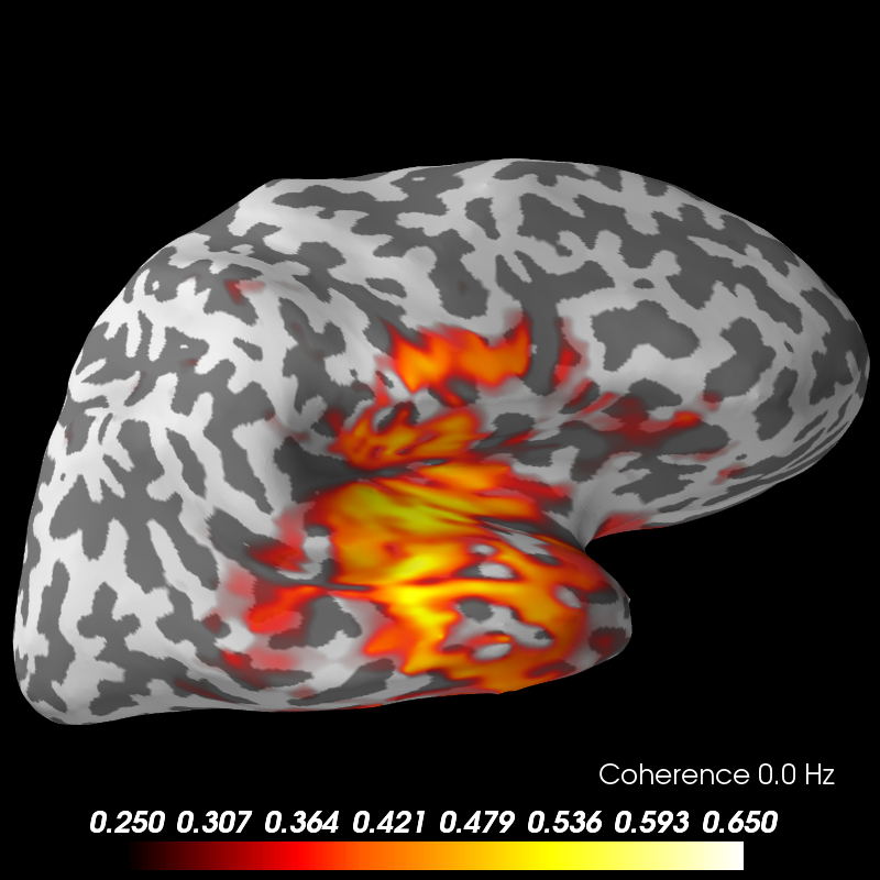
This examples computes the coherence between a seed in the left auditory cortex and the rest of the brain based on single-trial MNE-dSPM inverse solutions.
Out:
Reading inverse operator decomposition from /home/ubuntu/mne_data/MNE-sample-data/MEG/sample/sample_audvis-meg-oct-6-meg-inv.fif...
    Reading inverse operator info...
    [done]
    Reading inverse operator decomposition...
    [done]
    305 x 305 full covariance (kind = 1) found.
    Read a total of 4 projection items:
        PCA-v1 (1 x 10²) active
        PCA-v2 (1 x 10²) active
        PCA-v3 (1 x 10²) active
        Average EEG reference (1 x 60) active
    Noise covariance matrix read.
    22494 x 22494 diagonal covariance (kind = 2) found.
    Source covariance matrix read.
    22494 x 22494 diagonal covariance (kind = 6) found.
    Orientation priors read.
    22494 x 22494 diagonal covariance (kind = 5) found.
    Depth priors read.
    Did not find the desired covariance matrix (kind = 3)
    Reading a source space...
    Computing patch statistics...
    Patch information added...
    Distance information added...
    [done]
    Reading a source space...
    Computing patch statistics...
    Patch information added...
    Distance information added...
    [done]
    2 source spaces read
    Read a total of 4 projection items:
        PCA-v1 (1 x 10²) active
        PCA-v2 (1 x 10²) active
        PCA-v3 (1 x 10²) active
        Average EEG reference (1 x 60) active
    Source spaces transformed to the inverse solution coordinate frame
Opening raw data file /home/ubuntu/mne_data/MNE-sample-data/MEG/sample/sample_audvis_filt-0-40_raw.fif...
    Read a total of 4 projection items:
        PCA-v1 (1 x 10²)  idle
        PCA-v2 (1 x 10²)  idle
        PCA-v3 (1 x 10²)  idle
        Average EEG reference (1 x 60)  idle
    Range : 6450 ... 48149 =     42.956 ...   320.665 secs
Ready.
Current compensation grade : 0
72 matching events found
Created an SSP operator (subspace dimension = 3)
4 projection items activated
    Rejecting  epoch based on EOG : [u'EOG 061']
    Rejecting  epoch based on EOG : [u'EOG 061']
    Rejecting  epoch based on EOG : [u'EOG 061']
    Rejecting  epoch based on EOG : [u'EOG 061']
    Rejecting  epoch based on EOG : [u'EOG 061']
    Rejecting  epoch based on MAG : [u'MEG 1711']
    Rejecting  epoch based on EOG : [u'EOG 061']
    Rejecting  epoch based on EOG : [u'EOG 061']
    Rejecting  epoch based on EOG : [u'EOG 061']
    Rejecting  epoch based on EOG : [u'EOG 061']
    Rejecting  epoch based on EOG : [u'EOG 061']
    Rejecting  epoch based on EOG : [u'EOG 061']
    Rejecting  epoch based on EOG : [u'EOG 061']
    Rejecting  epoch based on EOG : [u'EOG 061']
    Rejecting  epoch based on EOG : [u'EOG 061']
    Rejecting  epoch based on EOG : [u'EOG 061']
    Rejecting  epoch based on EOG : [u'EOG 061']
Preparing the inverse operator for use...
    Scaled noise and source covariance from nave = 1 to nave = 55
    Created the regularized inverter
    Created an SSP operator (subspace dimension = 3)
    Created the whitener using a full noise covariance matrix (3 small eigenvalues omitted)
    Computing noise-normalization factors (dSPM)...
[done]
Picked 305 channels from the data
Computing inverse...
(eigenleads need to be weighted)...
(dSPM)...
[done]
Connectivity computation...
Preparing the inverse operator for use...
    Scaled noise and source covariance from nave = 1 to nave = 1
    Created the regularized inverter
    Created an SSP operator (subspace dimension = 3)
    Created the whitener using a full noise covariance matrix (3 small eigenvalues omitted)
    Computing noise-normalization factors (dSPM)...
[done]
Picked 305 channels from the data
Computing inverse...
(eigenleads need to be weighted)...
Processing epoch : 1
    computing connectivity for 7498 connections
    using t=-0.200s..0.499s for estimation (106 points)
    computing connectivity for the bands:
     band 1: 8.5Hz..12.7Hz (4 points)
     band 2: 14.2Hz..29.7Hz (12 points)
    connectivity scores will be averaged for each band
    using FFT with a Hanning window to estimate spectra
    the following metrics will be computed: Coherence
    computing connectivity for epoch 1
Processing epoch : 2
    computing connectivity for epoch 2
Processing epoch : 3
    computing connectivity for epoch 3
Processing epoch : 4
    computing connectivity for epoch 4
Processing epoch : 5
    computing connectivity for epoch 5
Processing epoch : 6
    computing connectivity for epoch 6
Processing epoch : 7
    computing connectivity for epoch 7
Processing epoch : 8
    computing connectivity for epoch 8
Processing epoch : 9
    computing connectivity for epoch 9
Processing epoch : 10
    computing connectivity for epoch 10
    Rejecting  epoch based on EOG : [u'EOG 061']
Processing epoch : 11
    computing connectivity for epoch 11
Processing epoch : 12
    computing connectivity for epoch 12
Processing epoch : 13
    computing connectivity for epoch 13
    Rejecting  epoch based on EOG : [u'EOG 061']
    Rejecting  epoch based on EOG : [u'EOG 061']
Processing epoch : 14
    computing connectivity for epoch 14
Processing epoch : 15
    computing connectivity for epoch 15
Processing epoch : 16
    computing connectivity for epoch 16
Processing epoch : 17
    computing connectivity for epoch 17
    Rejecting  epoch based on EOG : [u'EOG 061']
Processing epoch : 18
    computing connectivity for epoch 18
Processing epoch : 19
    computing connectivity for epoch 19
Processing epoch : 20
    computing connectivity for epoch 20
    Rejecting  epoch based on EOG : [u'EOG 061']
Processing epoch : 21
    computing connectivity for epoch 21
Processing epoch : 22
    computing connectivity for epoch 22
Processing epoch : 23
    computing connectivity for epoch 23
    Rejecting  epoch based on MAG : [u'MEG 1711']
Processing epoch : 24
    computing connectivity for epoch 24
Processing epoch : 25
    computing connectivity for epoch 25
Processing epoch : 26
    computing connectivity for epoch 26
Processing epoch : 27
    computing connectivity for epoch 27
Processing epoch : 28
    computing connectivity for epoch 28
    Rejecting  epoch based on EOG : [u'EOG 061']
Processing epoch : 29
    computing connectivity for epoch 29
Processing epoch : 30
    computing connectivity for epoch 30
Processing epoch : 31
    computing connectivity for epoch 31
    Rejecting  epoch based on EOG : [u'EOG 061']
Processing epoch : 32
    computing connectivity for epoch 32
Processing epoch : 33
    computing connectivity for epoch 33
    Rejecting  epoch based on EOG : [u'EOG 061']
Processing epoch : 34
    computing connectivity for epoch 34
Processing epoch : 35
    computing connectivity for epoch 35
    Rejecting  epoch based on EOG : [u'EOG 061']
    Rejecting  epoch based on EOG : [u'EOG 061']
Processing epoch : 36
    computing connectivity for epoch 36
    Rejecting  epoch based on EOG : [u'EOG 061']
    Rejecting  epoch based on EOG : [u'EOG 061']
Processing epoch : 37
    computing connectivity for epoch 37
Processing epoch : 38
    computing connectivity for epoch 38
Processing epoch : 39
    computing connectivity for epoch 39
Processing epoch : 40
    computing connectivity for epoch 40
Processing epoch : 41
    computing connectivity for epoch 41
Processing epoch : 42
    computing connectivity for epoch 42
Processing epoch : 43
    computing connectivity for epoch 43
Processing epoch : 44
    computing connectivity for epoch 44
    Rejecting  epoch based on EOG : [u'EOG 061']
Processing epoch : 45
    computing connectivity for epoch 45
    Rejecting  epoch based on EOG : [u'EOG 061']
Processing epoch : 46
    computing connectivity for epoch 46
Processing epoch : 47
    computing connectivity for epoch 47
Processing epoch : 48
    computing connectivity for epoch 48
    Rejecting  epoch based on EOG : [u'EOG 061']
    Rejecting  epoch based on EOG : [u'EOG 061']
Processing epoch : 49
    computing connectivity for epoch 49
Processing epoch : 50
    computing connectivity for epoch 50
Processing epoch : 51
    computing connectivity for epoch 51
Processing epoch : 52
    computing connectivity for epoch 52
Processing epoch : 53
    computing connectivity for epoch 53
Processing epoch : 54
    computing connectivity for epoch 54
Processing epoch : 55
    computing connectivity for epoch 55
[done]
[Connectivity computation done]
Frequencies in Hz over which coherence was averaged for alpha:
[  8.49926873   9.91581352  11.33235831  12.74890309]
Frequencies in Hz over which coherence was averaged for beta:
[ 14.16544788  15.58199267  16.99853746  18.41508225  19.83162704
  21.24817182  22.66471661  24.0812614   25.49780619  26.91435098
  28.33089577  29.74744055]
Updating smoothing matrix, be patient..
Smoothing matrix creation, step 1
Smoothing matrix creation, step 2
Smoothing matrix creation, step 3
Smoothing matrix creation, step 4
Smoothing matrix creation, step 5
Smoothing matrix creation, step 6
Smoothing matrix creation, step 7
Smoothing matrix creation, step 8
Smoothing matrix creation, step 9
Smoothing matrix creation, step 10
colormap: fmin=2.50e-01 fmid=4.00e-01 fmax=6.50e-01 transparent=1
# Author: Martin Luessi <mluessi@nmr.mgh.harvard.edu>
#
# License: BSD (3-clause)

import numpy as np

import mne
from mne.datasets import sample
from mne.minimum_norm import (apply_inverse, apply_inverse_epochs,
                              read_inverse_operator)
from mne.connectivity import seed_target_indices, spectral_connectivity

print(__doc__)

data_path = sample.data_path()
subjects_dir = data_path + '/subjects'
fname_inv = data_path + '/MEG/sample/sample_audvis-meg-oct-6-meg-inv.fif'
fname_raw = data_path + '/MEG/sample/sample_audvis_filt-0-40_raw.fif'
fname_event = data_path + '/MEG/sample/sample_audvis_filt-0-40_raw-eve.fif'
label_name_lh = 'Aud-lh'
fname_label_lh = data_path + '/MEG/sample/labels/%s.label' % label_name_lh

event_id, tmin, tmax = 1, -0.2, 0.5
method = "dSPM"  # use dSPM method (could also be MNE or sLORETA)

# Load data.
inverse_operator = read_inverse_operator(fname_inv)
label_lh = mne.read_label(fname_label_lh)
raw = mne.io.read_raw_fif(fname_raw)
events = mne.read_events(fname_event)

# Add a bad channel.
raw.info['bads'] += ['MEG 2443']

# pick MEG channels.
picks = mne.pick_types(raw.info, meg=True, eeg=False, stim=False, eog=True,
                       exclude='bads')

# Read epochs.
epochs = mne.Epochs(raw, events, event_id, tmin, tmax, picks=picks,
                    baseline=(None, 0),
                    reject=dict(mag=4e-12, grad=4000e-13, eog=150e-6))

# First, we find the most active vertex in the left auditory cortex, which
# we will later use as seed for the connectivity computation.
snr = 3.0
lambda2 = 1.0 / snr ** 2
evoked = epochs.average()
stc = apply_inverse(evoked, inverse_operator, lambda2, method,
                    pick_ori="normal")

# Restrict the source estimate to the label in the left auditory cortex.
stc_label = stc.in_label(label_lh)

# Find number and index of vertex with most power.
src_pow = np.sum(stc_label.data ** 2, axis=1)
seed_vertno = stc_label.vertices[0][np.argmax(src_pow)]
seed_idx = np.searchsorted(stc.vertices[0], seed_vertno)  # index in orig stc

# Generate index parameter for seed-based connectivity analysis.
n_sources = stc.data.shape[0]
indices = seed_target_indices([seed_idx], np.arange(n_sources))

# Compute inverse solution and for each epoch. By using "return_generator=True"
# stcs will be a generator object instead of a list. This allows us so to
# compute the coherence without having to keep all source estimates in memory.

snr = 1.0  # use lower SNR for single epochs
lambda2 = 1.0 / snr ** 2
stcs = apply_inverse_epochs(epochs, inverse_operator, lambda2, method,
                            pick_ori="normal", return_generator=True)

# Now we are ready to compute the coherence in the alpha and beta band.
# fmin and fmax specify the lower and upper freq. for each band, resp.
fmin = (8., 13.)
fmax = (13., 30.)
sfreq = raw.info['sfreq']  # the sampling frequency

# Now we compute connectivity. To speed things up, we use 2 parallel jobs
# and use mode='fourier', which uses a FFT with a Hanning window
# to compute the spectra (instead of multitaper estimation, which has a
# lower variance but is slower). By using faverage=True, we directly
# average the coherence in the alpha and beta band, i.e., we will only
# get 2 frequency bins.
coh, freqs, times, n_epochs, n_tapers = spectral_connectivity(
    stcs, method='coh', mode='fourier', indices=indices,
    sfreq=sfreq, fmin=fmin, fmax=fmax, faverage=True, n_jobs=1)

print('Frequencies in Hz over which coherence was averaged for alpha: ')
print(freqs[0])
print('Frequencies in Hz over which coherence was averaged for beta: ')
print(freqs[1])

# Generate a SourceEstimate with the coherence. This is simple since we
# used a single seed. For more than one seeds we would have to split coh.
# Note: We use a hack to save the frequency axis as time.
tmin = np.mean(freqs[0])
tstep = np.mean(freqs[1]) - tmin
coh_stc = mne.SourceEstimate(coh, vertices=stc.vertices, tmin=1e-3 * tmin,
                             tstep=1e-3 * tstep, subject='sample')

# Now we can visualize the coherence using the plot method.
brain = coh_stc.plot('sample', 'inflated', 'both',
                     time_label='Coherence %0.1f Hz',
                     subjects_dir=subjects_dir,
                     clim=dict(kind='value', lims=(0.25, 0.4, 0.65)))
brain.show_view('lateral')
Total running time of the script: ( 0 minutes 40.514 seconds)