Decoding in sensor space data using the Common Spatial Pattern (CSP)¶

# Authors: Alexandre Gramfort <alexandre.gramfort@telecom-paristech.fr>
#          Romain Trachel <romain.trachel@inria.fr>
#
# License: BSD (3-clause)

import numpy as np
import matplotlib.pyplot as plt

import mne
from mne import io
from mne.datasets import sample

print(__doc__)

data_path = sample.data_path()

raw_fname = data_path + '/MEG/sample/sample_audvis_filt-0-40_raw.fif'
event_fname = data_path + '/MEG/sample/sample_audvis_filt-0-40_raw-eve.fif'
tmin, tmax = -0.2, 0.5
event_id = dict(aud_l=1, vis_l=3)

# Setup for reading the raw data
raw = io.read_raw_fif(raw_fname, preload=True)
raw.filter(2, None)  # replace baselining with high-pass
events = mne.read_events(event_fname)

raw.info['bads'] = ['MEG 2443']  # set bad channels
picks = mne.pick_types(raw.info, meg='grad', eeg=False, stim=False, eog=False,
                       exclude='bads')

# Read epochs
epochs = mne.Epochs(raw, events, event_id, tmin, tmax, proj=True,
                    picks=picks, baseline=None, preload=True)

labels = epochs.events[:, -1]
evoked = epochs.average()

from sklearn.svm import SVC  # noqa
from sklearn.cross_validation import ShuffleSplit  # noqa
from mne.decoding import CSP  # noqa

n_components = 3  # pick some components
svc = SVC(C=1, kernel='linear')
csp = CSP(n_components=n_components)

# Define a monte-carlo cross-validation generator (reduce variance):
cv = ShuffleSplit(len(labels), 10, test_size=0.2, random_state=42)
scores = []
epochs_data = epochs.get_data()

for train_idx, test_idx in cv:
    y_train, y_test = labels[train_idx], labels[test_idx]

    X_train = csp.fit_transform(epochs_data[train_idx], y_train)
    X_test = csp.transform(epochs_data[test_idx])

    # fit classifier
    svc.fit(X_train, y_train)

    scores.append(svc.score(X_test, y_test))

# Printing the results
class_balance = np.mean(labels == labels[0])
class_balance = max(class_balance, 1. - class_balance)
print("Classification accuracy: %f / Chance level: %f" % (np.mean(scores),
                                                          class_balance))

# Or use much more convenient scikit-learn cross_val_score function using
# a Pipeline
from sklearn.pipeline import Pipeline  # noqa
from sklearn.cross_validation import cross_val_score  # noqa
cv = ShuffleSplit(len(labels), 10, test_size=0.2, random_state=42)
clf = Pipeline([('CSP', csp), ('SVC', svc)])
scores = cross_val_score(clf, epochs_data, labels, cv=cv, n_jobs=1)
print(scores.mean())  # should match results above

# And using reuglarized csp with Ledoit-Wolf estimator
csp = CSP(n_components=n_components, reg='ledoit_wolf')
clf = Pipeline([('CSP', csp), ('SVC', svc)])
scores = cross_val_score(clf, epochs_data, labels, cv=cv, n_jobs=1)
print(scores.mean())  # should get better results than above

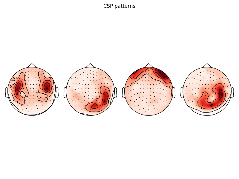
# plot CSP patterns estimated on full data for visualization
csp.fit_transform(epochs_data, labels)
data = csp.patterns_
fig, axes = plt.subplots(1, 4)
for idx in range(4):
    mne.viz.plot_topomap(data[idx], evoked.info, axes=axes[idx], show=False)
fig.suptitle('CSP patterns')
fig.tight_layout()
fig.show()