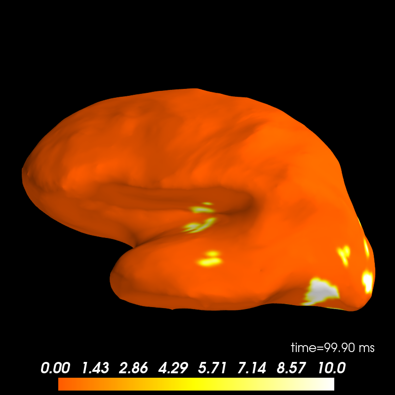
Decoding, a.k.a MVPA or supervised machine learning applied to MEG data in source space on the left cortical surface. Here f-test feature selection is employed to confine the classification to the potentially relevant features. The classifier then is trained to selected features of epochs in source space.
# Author: Denis A. Engemann <denis.engemann@gmail.com>
#         Alexandre Gramfort <alexandre.gramfort@telecom-paristech.fr>
#
# License: BSD (3-clause)

import mne
import os
import numpy as np
from mne import io
from mne.datasets import sample
from mne.minimum_norm import apply_inverse_epochs, read_inverse_operator

print(__doc__)

data_path = sample.data_path()
fname_fwd = data_path + 'MEG/sample/sample_audvis-meg-oct-6-fwd.fif'
fname_evoked = data_path + '/MEG/sample/sample_audvis-ave.fif'
subjects_dir = data_path + '/subjects'
subject = os.environ['SUBJECT'] = subjects_dir + '/sample'
os.environ['SUBJECTS_DIR'] = subjects_dir
Set parameters
raw_fname = data_path + '/MEG/sample/sample_audvis_filt-0-40_raw.fif'
event_fname = data_path + '/MEG/sample/sample_audvis_filt-0-40_raw-eve.fif'
fname_cov = data_path + '/MEG/sample/sample_audvis-cov.fif'
label_names = 'Aud-rh', 'Vis-rh'
fname_inv = data_path + '/MEG/sample/sample_audvis-meg-oct-6-meg-inv.fif'

tmin, tmax = -0.2, 0.5
event_id = dict(aud_r=2, vis_r=4)  # load contra-lateral conditions

# Setup for reading the raw data
raw = io.read_raw_fif(raw_fname, preload=True)
raw.filter(2, None)  # replace baselining with high-pass
events = mne.read_events(event_fname)

# Set up pick list: MEG - bad channels (modify to your needs)
raw.info['bads'] += ['MEG 2443']  # mark bads
picks = mne.pick_types(raw.info, meg=True, eeg=False, stim=True, eog=True,
                       exclude='bads')

# Read epochs
epochs = mne.Epochs(raw, events, event_id, tmin, tmax, proj=True,
                    picks=picks, baseline=None, preload=True,
                    reject=dict(grad=4000e-13, eog=150e-6),
                    decim=5)  # decimate to save memory and increase speed

epochs.equalize_event_counts(list(event_id.keys()))
epochs_list = [epochs[k] for k in event_id]

# Compute inverse solution
snr = 3.0
lambda2 = 1.0 / snr ** 2
method = "dSPM"  # use dSPM method (could also be MNE or sLORETA)
n_times = len(epochs.times)
n_vertices = 3732
n_epochs = len(epochs.events)

# Load data and compute inverse solution and stcs for each epoch.

noise_cov = mne.read_cov(fname_cov)
inverse_operator = read_inverse_operator(fname_inv)
X = np.zeros([n_epochs, n_vertices, n_times])

# to save memory, we'll load and transform our epochs step by step.
for condition_count, ep in zip([0, n_epochs // 2], epochs_list):
    stcs = apply_inverse_epochs(ep, inverse_operator, lambda2,
                                method, pick_ori="normal",  # saves us memory
                                return_generator=True)
    for jj, stc in enumerate(stcs):
        X[condition_count + jj] = stc.lh_data
Out:
Opening raw data file /home/ubuntu/mne_data/MNE-sample-data/MEG/sample/sample_audvis_filt-0-40_raw.fif...
    Read a total of 4 projection items:
        PCA-v1 (1 x 10²)  idle
        PCA-v2 (1 x 10²)  idle
        PCA-v3 (1 x 10²)  idle
        Average EEG reference (1 x 60)  idle
    Range : 6450 ... 48149 =     42.956 ...   320.665 secs
Ready.
Current compensation grade : 0
Reading 0 ... 41699  =      0.000 ...   277.709 secs...
Setting up high-pass filter at 2 Hz
l_trans_bandwidth chosen to be 2.0 Hz
Filter length of 496 samples (3.303 sec) selected
143 matching events found
The measurement information indicates a low-pass frequency of 40 Hz. The decim=5 parameter will result in a sampling frequency of 30.0307 Hz, which can cause aliasing artifacts.
Created an SSP operator (subspace dimension = 3)
4 projection items activated
Loading data for 143 events and 106 original time points ...
    Rejecting  epoch based on EOG : [u'EOG 061']
    Rejecting  epoch based on EOG : [u'EOG 061']
    Rejecting  epoch based on EOG : [u'EOG 061']
    Rejecting  epoch based on EOG : [u'EOG 061']
    Rejecting  epoch based on EOG : [u'EOG 061']
    Rejecting  epoch based on EOG : [u'EOG 061']
    Rejecting  epoch based on EOG : [u'EOG 061']
    Rejecting  epoch based on EOG : [u'EOG 061']
    Rejecting  epoch based on EOG : [u'EOG 061']
    Rejecting  epoch based on EOG : [u'EOG 061']
    Rejecting  epoch based on EOG : [u'EOG 061']
    Rejecting  epoch based on EOG : [u'EOG 061']
    Rejecting  epoch based on EOG : [u'EOG 061']
    Rejecting  epoch based on EOG : [u'EOG 061']
    Rejecting  epoch based on EOG : [u'EOG 061']
    Rejecting  epoch based on EOG : [u'EOG 061']
    Rejecting  epoch based on EOG : [u'EOG 061']
    Rejecting  epoch based on EOG : [u'EOG 061']
    Rejecting  epoch based on EOG : [u'EOG 061']
    Rejecting  epoch based on EOG : [u'EOG 061']
    Rejecting  epoch based on EOG : [u'EOG 061']
    Rejecting  epoch based on EOG : [u'EOG 061']
    Rejecting  epoch based on EOG : [u'EOG 061']
    Rejecting  epoch based on EOG : [u'EOG 061']
    Rejecting  epoch based on EOG : [u'EOG 061']
25 bad epochs dropped
Dropped 6 epochs
    366 x 366 full covariance (kind = 1) found.
    Read a total of 4 projection items:
        PCA-v1 (1 x 10²) active
        PCA-v2 (1 x 10²) active
        PCA-v3 (1 x 10²) active
        Average EEG reference (1 x 60) active
Reading inverse operator decomposition from /home/ubuntu/mne_data/MNE-sample-data/MEG/sample/sample_audvis-meg-oct-6-meg-inv.fif...
    Reading inverse operator info...
    [done]
    Reading inverse operator decomposition...
    [done]
    305 x 305 full covariance (kind = 1) found.
    Read a total of 4 projection items:
        PCA-v1 (1 x 10²) active
        PCA-v2 (1 x 10²) active
        PCA-v3 (1 x 10²) active
        Average EEG reference (1 x 60) active
    Noise covariance matrix read.
    22494 x 22494 diagonal covariance (kind = 2) found.
    Source covariance matrix read.
    22494 x 22494 diagonal covariance (kind = 6) found.
    Orientation priors read.
    22494 x 22494 diagonal covariance (kind = 5) found.
    Depth priors read.
    Did not find the desired covariance matrix (kind = 3)
    Reading a source space...
    Computing patch statistics...
    Patch information added...
    Distance information added...
    [done]
    Reading a source space...
    Computing patch statistics...
    Patch information added...
    Distance information added...
    [done]
    2 source spaces read
    Read a total of 4 projection items:
        PCA-v1 (1 x 10²) active
        PCA-v2 (1 x 10²) active
        PCA-v3 (1 x 10²) active
        Average EEG reference (1 x 60) active
    Source spaces transformed to the inverse solution coordinate frame
Preparing the inverse operator for use...
    Scaled noise and source covariance from nave = 1 to nave = 1
    Created the regularized inverter
    Created an SSP operator (subspace dimension = 3)
    Created the whitener using a full noise covariance matrix (3 small eigenvalues omitted)
    Computing noise-normalization factors (dSPM)...
[done]
Picked 305 channels from the data
Computing inverse...
(eigenleads need to be weighted)...
Processing epoch : 1
Processing epoch : 2
Processing epoch : 3
Processing epoch : 4
Processing epoch : 5
Processing epoch : 6
Processing epoch : 7
Processing epoch : 8
Processing epoch : 9
Processing epoch : 10
Processing epoch : 11
Processing epoch : 12
Processing epoch : 13
Processing epoch : 14
Processing epoch : 15
Processing epoch : 16
Processing epoch : 17
Processing epoch : 18
Processing epoch : 19
Processing epoch : 20
Processing epoch : 21
Processing epoch : 22
Processing epoch : 23
Processing epoch : 24
Processing epoch : 25
Processing epoch : 26
Processing epoch : 27
Processing epoch : 28
Processing epoch : 29
Processing epoch : 30
Processing epoch : 31
Processing epoch : 32
Processing epoch : 33
Processing epoch : 34
Processing epoch : 35
Processing epoch : 36
Processing epoch : 37
Processing epoch : 38
Processing epoch : 39
Processing epoch : 40
Processing epoch : 41
Processing epoch : 42
Processing epoch : 43
Processing epoch : 44
Processing epoch : 45
Processing epoch : 46
Processing epoch : 47
Processing epoch : 48
Processing epoch : 49
Processing epoch : 50
Processing epoch : 51
Processing epoch : 52
Processing epoch : 53
Processing epoch : 54
Processing epoch : 55
Processing epoch : 56
[done]
Decoding in sensor space using a linear SVM
# Make arrays X and y such that :
# X is 3d with X.shape[0] is the total number of epochs to classify
# y is filled with integers coding for the class to predict
# We must have X.shape[0] equal to y.shape[0]

# we know the first half belongs to the first class, the second one
y = np.repeat([0, 1], len(X) / 2)   # belongs to the second class
X = X.reshape(n_epochs, n_vertices * n_times)
# we have to normalize the data before supplying them to our classifier
X -= X.mean(axis=0)
X /= X.std(axis=0)

# prepare classifier
from sklearn.svm import SVC  # noqa
from sklearn.cross_validation import ShuffleSplit  # noqa

# Define a monte-carlo cross-validation generator (reduce variance):
n_splits = 10
clf = SVC(C=1, kernel='linear')
cv = ShuffleSplit(len(X), n_splits, test_size=0.2)

# setup feature selection and classification pipeline
from sklearn.feature_selection import SelectKBest, f_classif  # noqa
from sklearn.pipeline import Pipeline  # noqa

# we will use an ANOVA f-test to preselect relevant spatio-temporal units
feature_selection = SelectKBest(f_classif, k=500)  # take the best 500
# to make life easier we will create a pipeline object
anova_svc = Pipeline([('anova', feature_selection), ('svc', clf)])

# initialize score and feature weights result arrays
scores = np.zeros(n_splits)
feature_weights = np.zeros([n_vertices, n_times])

# hold on, this may take a moment
for ii, (train, test) in enumerate(cv):
    anova_svc.fit(X[train], y[train])
    y_pred = anova_svc.predict(X[test])
    y_test = y[test]
    scores[ii] = np.sum(y_pred == y_test) / float(len(y_test))
    feature_weights += feature_selection.inverse_transform(clf.coef_) \
        .reshape(n_vertices, n_times)

print('Average prediction accuracy: %0.3f | standard deviation:  %0.3f'
      % (scores.mean(), scores.std()))

# prepare feature weights for visualization
feature_weights /= (ii + 1)  # create average weights
# create mask to avoid division error
feature_weights = np.ma.masked_array(feature_weights, feature_weights == 0)
# normalize scores for visualization purposes
feature_weights /= feature_weights.std(axis=1)[:, None]
feature_weights -= feature_weights.mean(axis=1)[:, None]

# unmask, take absolute values, emulate f-value scale
feature_weights = np.abs(feature_weights.data) * 10

vertices = [stc.lh_vertno, np.array([], int)]  # empty array for right hemi
stc_feat = mne.SourceEstimate(feature_weights, vertices=vertices,
                              tmin=stc.tmin, tstep=stc.tstep,
                              subject='sample')

brain = stc_feat.plot(views=['lat'], transparent=True,
                      initial_time=0.1, time_unit='s')
Out:
Average prediction accuracy: 0.978 | standard deviation:  0.022
Updating smoothing matrix, be patient..
Smoothing matrix creation, step 1
Smoothing matrix creation, step 2
Smoothing matrix creation, step 3
Smoothing matrix creation, step 4
Smoothing matrix creation, step 5
Smoothing matrix creation, step 6
Smoothing matrix creation, step 7
Smoothing matrix creation, step 8
Smoothing matrix creation, step 9
Smoothing matrix creation, step 10
colormap: fmin=0.00e+00 fmid=1.00e-04 fmax=1.00e+01 transparent=1
Total running time of the script: ( 0 minutes 17.012 seconds)