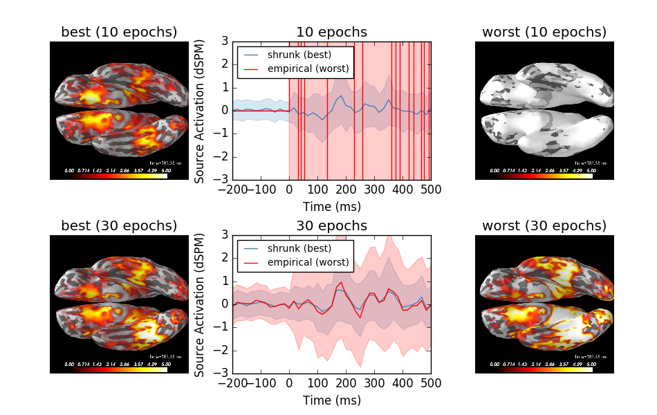
This example demonstrates the relationship between the noise covariance estimate and the MNE / dSPM source amplitudes. It computes source estimates for the SPM faces data and compares proper regularization with insufficient regularization based on the methods described in [1]. The example demonstrates that improper regularization can lead to overestimation of source amplitudes. This example makes use of the previous, non-optimized code path that was used before implementing the suggestions presented in [1]. Please do not copy the patterns presented here for your own analysis, this is example is purely illustrative.
Note
This example does quite a bit of processing, so even on a fast machine it can take a couple of minutes to complete.
| [1] | (1, 2) Engemann D. and Gramfort A. (2015) Automated model selection in covariance estimation and spatial whitening of MEG and EEG signals, vol. 108, 328-342, NeuroImage. |
# Author: Denis A. Engemann <denis.engemann@gmail.com>
#
# License: BSD (3-clause)

import os
import os.path as op

import numpy as np
from scipy.misc import imread
import matplotlib.pyplot as plt

import mne
from mne import io
from mne.datasets import spm_face
from mne.minimum_norm import apply_inverse, make_inverse_operator
from mne.cov import compute_covariance

print(__doc__)
Get data
data_path = spm_face.data_path()
subjects_dir = data_path + '/subjects'

raw_fname = data_path + '/MEG/spm/SPM_CTF_MEG_example_faces%d_3D.ds'

raw = io.read_raw_ctf(raw_fname % 1)  # Take first run
# To save time and memory for this demo, we'll just use the first
# 2.5 minutes (all we need to get 30 total events) and heavily
# resample 480->60 Hz (usually you wouldn't do either of these!)
raw = raw.crop(0, 150.).load_data().resample(60, npad='auto')

picks = mne.pick_types(raw.info, meg=True, exclude='bads')
raw.filter(1, None, n_jobs=1)

events = mne.find_events(raw, stim_channel='UPPT001')

event_ids = {"faces": 1, "scrambled": 2}
tmin, tmax = -0.2, 0.5
baseline = None  # no baseline as high-pass is applied
reject = dict(mag=3e-12)

# Make source space

trans = data_path + '/MEG/spm/SPM_CTF_MEG_example_faces1_3D_raw-trans.fif'
src = mne.setup_source_space('spm', fname=None, spacing='oct6',
                             subjects_dir=subjects_dir, add_dist=False)
bem = data_path + '/subjects/spm/bem/spm-5120-5120-5120-bem-sol.fif'
forward = mne.make_forward_solution(raw.info, trans, src, bem)
forward = mne.convert_forward_solution(forward, surf_ori=True)
del src

# inverse parameters
conditions = 'faces', 'scrambled'
snr = 3.0
lambda2 = 1.0 / snr ** 2
method = 'dSPM'
clim = dict(kind='value', lims=[0, 2.5, 5])
Out:
ds directory : /home/ubuntu/mne_data/MNE-spm-face/MEG/spm/SPM_CTF_MEG_example_faces1_3D.ds
    res4 data read.
    hc data read.
    Separate EEG position data file not present.
    Quaternion matching (desired vs. transformed):
      -0.90   72.01    0.00 mm <->   -0.90   72.01    0.00 mm (orig :  -43.09   61.46 -252.17 mm) diff =    0.000 mm
       0.90  -72.01    0.00 mm <->    0.90  -72.01    0.00 mm (orig :   53.49  -45.24 -258.02 mm) diff =    0.000 mm
      98.30    0.00    0.00 mm <->   98.30   -0.00    0.00 mm (orig :   78.60   72.16 -241.87 mm) diff =    0.000 mm
    Coordinate transformations established.
    Polhemus data for 3 HPI coils added
    Device coordinate locations for 3 HPI coils added
    Measurement info composed.
Finding samples for /home/ubuntu/mne_data/MNE-spm-face/MEG/spm/SPM_CTF_MEG_example_faces1_3D.ds/SPM_CTF_MEG_example_faces1_3D.meg4:
    System clock channel is available, checking which samples are valid.
    1 x 324474 = 324474 samples from 340 chs
Current compensation grade : 3
Reading 0 ... 72000  =      0.000 ...   150.000 secs...
Setting up high-pass filter at 1 Hz
l_trans_bandwidth chosen to be 1.0 Hz
Filter length of 396 samples (6.600 sec) selected
41 events found
Events id: [1 2 3]
Setting up the source space with the following parameters:

SUBJECTS_DIR = /home/ubuntu/mne_data/MNE-spm-face/subjects
Subject      = spm
Surface      = white
Octahedron subdivision grade 6

>>> 1. Creating the source space...

Doing the octahedral vertex picking...
Loading /home/ubuntu/mne_data/MNE-spm-face/subjects/spm/surf/lh.white...
Mapping lh spm -> oct (6) ...
    Triangle neighbors and vertex normals...
Loading geometry from /home/ubuntu/mne_data/MNE-spm-face/subjects/spm/surf/lh.sphere...
    Triangle neighbors and vertex normals...
Setting up the triangulation for the decimated surface...
loaded lh.white 4098/139164 selected to source space (oct = 6)

Loading /home/ubuntu/mne_data/MNE-spm-face/subjects/spm/surf/rh.white...
Mapping rh spm -> oct (6) ...
    Triangle neighbors and vertex normals...
Loading geometry from /home/ubuntu/mne_data/MNE-spm-face/subjects/spm/surf/rh.sphere...
    Triangle neighbors and vertex normals...
Setting up the triangulation for the decimated surface...
loaded rh.white 4098/137848 selected to source space (oct = 6)

You are now one step closer to computing the gain matrix
Source space                 : <SourceSpaces: [<surface (lh), n_vertices=139164, n_used=4098, coordinate_frame=MRI (surface RAS)>, <surface (rh), n_vertices=137848, n_used=4098, coordinate_frame=MRI (surface RAS)>]>
MRI -> head transform source : /home/ubuntu/mne_data/MNE-spm-face/MEG/spm/SPM_CTF_MEG_example_faces1_3D_raw-trans.fif
Measurement data             : instance of Info
BEM model                    : /home/ubuntu/mne_data/MNE-spm-face/subjects/spm/bem/spm-5120-5120-5120-bem-sol.fif
Accurate field computations
Do computations in head coordinates
Free source orientations
Destination for the solution : None

Read 2 source spaces a total of 8196 active source locations

Coordinate transformation: MRI (surface RAS) -> head
     0.999622  0.006802  0.026647      -2.80 mm
    -0.014131  0.958276  0.285497       6.72 mm
    -0.023593 -0.285765  0.958009       9.43 mm
     0.000000  0.000000  0.000000       1.00

Read 274 MEG channels from info
Read  29 MEG compensation channels from info
81 coil definitions read
Coordinate transformation: MEG device -> head
     0.997940 -0.049681 -0.040594      -1.35 mm
     0.054745  0.989330  0.135013      -0.41 mm
     0.033453 -0.136957  0.990012      65.80 mm
     0.000000  0.000000  0.000000       1.00
5 compensation data sets in info
MEG coil definitions created in head coordinates.
Source spaces are now in head coordinates.

Setting up the BEM model using /home/ubuntu/mne_data/MNE-spm-face/subjects/spm/bem/spm-5120-5120-5120-bem-sol.fif...

Loading surfaces...
Three-layer model surfaces loaded.

Loading the solution matrix...

Loaded linear_collocation BEM solution from /home/ubuntu/mne_data/MNE-spm-face/subjects/spm/bem/spm-5120-5120-5120-bem-sol.fif
Employing the head->MRI coordinate transform with the BEM model.
BEM model spm-5120-5120-5120-bem-sol.fif is now set up

Source spaces are in head coordinates.
Checking that the sources are inside the bounding surface (will take a few...)
Thank you for waiting.

Setting up compensation data...
    274 out of 274 channels have the compensation set.
    Desired compensation data (3) found.
    All compensation channels found.
    Preselector created.
    Compensation data matrix created.
    Postselector created.

Composing the field computation matrix...
Composing the field computation matrix (compensation coils)...
Computing MEG at 8196 source locations (free orientations)...

Finished.
    Converting to surface-based source orientations...
[done]
Estimate covariances
samples_epochs = 5, 15,
method = 'empirical', 'shrunk'
colors = 'steelblue', 'red'

evokeds = list()
stcs = list()
methods_ordered = list()
for n_train in samples_epochs:
    # estimate covs based on a subset of samples
    # make sure we have the same number of conditions.
    events_ = np.concatenate([events[events[:, 2] == id_][:n_train]
                              for id_ in [event_ids[k] for k in conditions]])
    epochs_train = mne.Epochs(raw, events_, event_ids, tmin, tmax, picks=picks,
                              baseline=baseline, preload=True, reject=reject)
    epochs_train.equalize_event_counts(event_ids)
    assert len(epochs_train) == 2 * n_train

    noise_covs = compute_covariance(
        epochs_train, method=method, tmin=None, tmax=0,  # baseline only
        return_estimators=True)  # returns list
    # prepare contrast
    evokeds = [epochs_train[k].average() for k in conditions]
    del epochs_train, events_
    # do contrast

    # We skip empirical rank estimation that we introduced in response to
    # the findings in reference [1] to use the naive code path that
    # triggered the behavior described in [1]. The expected true rank is
    # 274 for this dataset. Please do not do this with your data but
    # rely on the default rank estimator that helps regularizing the
    # covariance.
    stcs.append(list())
    methods_ordered.append(list())
    for cov in noise_covs:
        inverse_operator = make_inverse_operator(evokeds[0].info, forward,
                                                 cov, loose=0.2, depth=0.8,
                                                 rank=274)
        stc_a, stc_b = (apply_inverse(e, inverse_operator, lambda2, "dSPM",
                                      pick_ori=None) for e in evokeds)
        stc = stc_a - stc_b
        methods_ordered[-1].append(cov['method'])
        stcs[-1].append(stc)
    del inverse_operator, evokeds, cov, noise_covs, stc, stc_a, stc_b
del raw, forward  # save some memory
Out:
The events passed to the Epochs constructor are not chronologically ordered.
10 matching events found
0 projection items activated
Loading data for 10 events and 43 original time points ...
0 bad epochs dropped
Dropped 0 epochs
Too few samples (required : 1375 got : 130), covariance estimate may be unreliable
Estimating covariance using EMPIRICAL
Done.
Estimating covariance using SHRUNK
Done.
Using cross-validation to select the best estimator.
Number of samples used : 130
[done]
Number of samples used : 130
[done]
log-likelihood on unseen data (descending order):
   shrunk: -1369.417
   empirical: -4039.119
Computing inverse operator with 274 channels.
Setting small MEG eigenvalues to zero.
Not doing PCA for MEG.
Total rank is 274
Creating the depth weighting matrix...
    274 magnetometer or axial gradiometer channels
    limit = 8109/8196 = 10.042069
    scale = 4.04483e-11 exp = 0.8
Computing inverse operator with 274 channels.
Creating the source covariance matrix
Applying loose dipole orientations. Loose value of 0.2.
Whitening the forward solution.
Adjusting source covariance matrix.
Computing SVD of whitened and weighted lead field matrix.
    largest singular value = 4.90761
    scaling factor to adjust the trace = 2.11023e+19
Preparing the inverse operator for use...
    Scaled noise and source covariance from nave = 1 to nave = 5
    Created the regularized inverter
    The projection vectors do not apply to these channels.
    Created the whitener using a full noise covariance matrix (0 small eigenvalues omitted)
    Computing noise-normalization factors (dSPM)...
[done]
Picked 274 channels from the data
Computing inverse...
(eigenleads need to be weighted)...
combining the current components...
(dSPM)...
[done]
Computing inverse operator with 274 channels.
Setting small MEG eigenvalues to zero.
Not doing PCA for MEG.
Total rank is 212
Creating the depth weighting matrix...
    274 magnetometer or axial gradiometer channels
    limit = 8109/8196 = 10.042069
    scale = 4.04483e-11 exp = 0.8
Computing inverse operator with 274 channels.
Creating the source covariance matrix
Applying loose dipole orientations. Loose value of 0.2.
Whitening the forward solution.
Adjusting source covariance matrix.
Computing SVD of whitened and weighted lead field matrix.
    largest singular value = 7.62283
    scaling factor to adjust the trace = 7.17196e+33
Preparing the inverse operator for use...
    Scaled noise and source covariance from nave = 1 to nave = 5
    Created the regularized inverter
    The projection vectors do not apply to these channels.
    Created the whitener using a full noise covariance matrix (62 small eigenvalues omitted)
    Computing noise-normalization factors (dSPM)...
[done]
Picked 274 channels from the data
Computing inverse...
(eigenleads need to be weighted)...
combining the current components...
(dSPM)...
[done]
The events passed to the Epochs constructor are not chronologically ordered.
30 matching events found
0 projection items activated
Loading data for 30 events and 43 original time points ...
0 bad epochs dropped
Dropped 0 epochs
Too few samples (required : 1375 got : 390), covariance estimate may be unreliable
Estimating covariance using EMPIRICAL
Done.
Estimating covariance using SHRUNK
Done.
Using cross-validation to select the best estimator.
Number of samples used : 390
[done]
Number of samples used : 390
[done]
log-likelihood on unseen data (descending order):
   shrunk: -1329.897
   empirical: -4079.150
Computing inverse operator with 274 channels.
Setting small MEG eigenvalues to zero.
Not doing PCA for MEG.
Total rank is 274
Creating the depth weighting matrix...
    274 magnetometer or axial gradiometer channels
    limit = 8109/8196 = 10.042069
    scale = 4.04483e-11 exp = 0.8
Computing inverse operator with 274 channels.
Creating the source covariance matrix
Applying loose dipole orientations. Loose value of 0.2.
Whitening the forward solution.
Adjusting source covariance matrix.
Computing SVD of whitened and weighted lead field matrix.
    largest singular value = 4.09049
    scaling factor to adjust the trace = 1.40662e+19
Preparing the inverse operator for use...
    Scaled noise and source covariance from nave = 1 to nave = 15
    Created the regularized inverter
    The projection vectors do not apply to these channels.
    Created the whitener using a full noise covariance matrix (0 small eigenvalues omitted)
    Computing noise-normalization factors (dSPM)...
[done]
Picked 274 channels from the data
Computing inverse...
(eigenleads need to be weighted)...
combining the current components...
(dSPM)...
[done]
Computing inverse operator with 274 channels.
Setting small MEG eigenvalues to zero.
Not doing PCA for MEG.
Total rank is 274
Creating the depth weighting matrix...
    274 magnetometer or axial gradiometer channels
    limit = 8109/8196 = 10.042069
    scale = 4.04483e-11 exp = 0.8
Computing inverse operator with 274 channels.
Creating the source covariance matrix
Applying loose dipole orientations. Loose value of 0.2.
Whitening the forward solution.
Adjusting source covariance matrix.
Computing SVD of whitened and weighted lead field matrix.
    largest singular value = 4.21107
    scaling factor to adjust the trace = 4.01968e+19
Preparing the inverse operator for use...
    Scaled noise and source covariance from nave = 1 to nave = 15
    Created the regularized inverter
    The projection vectors do not apply to these channels.
    Created the whitener using a full noise covariance matrix (0 small eigenvalues omitted)
    Computing noise-normalization factors (dSPM)...
[done]
Picked 274 channels from the data
Computing inverse...
(eigenleads need to be weighted)...
combining the current components...
(dSPM)...
[done]
Show the resulting source estimates
fig, (axes1, axes2) = plt.subplots(2, 3, figsize=(9.5, 6))


def brain_to_mpl(brain):
    """convert image to be usable with matplotlib"""
    tmp_path = op.abspath(op.join(op.curdir, 'my_tmp'))
    brain.save_imageset(tmp_path, views=['ven'])
    im = imread(tmp_path + '_ven.png')
    os.remove(tmp_path + '_ven.png')
    return im


for ni, (n_train, axes) in enumerate(zip(samples_epochs, (axes1, axes2))):
    # compute stc based on worst and best
    ax_dynamics = axes[1]
    for stc, ax, method, kind, color in zip(stcs[ni],
                                            axes[::2],
                                            methods_ordered[ni],
                                            ['best', 'worst'],
                                            colors):
        brain = stc.plot(subjects_dir=subjects_dir, hemi='both', clim=clim,
                         initial_time=0.175)

        im = brain_to_mpl(brain)
        brain.close()
        del brain
        ax.axis('off')
        ax.get_xaxis().set_visible(False)
        ax.get_yaxis().set_visible(False)
        ax.imshow(im)
        ax.set_title('{0} ({1} epochs)'.format(kind, n_train * 2))

        # plot spatial mean
        stc_mean = stc.data.mean(0)
        ax_dynamics.plot(stc.times * 1e3, stc_mean,
                         label='{0} ({1})'.format(method, kind),
                         color=color)
        # plot spatial std
        stc_var = stc.data.std(0)
        ax_dynamics.fill_between(stc.times * 1e3, stc_mean - stc_var,
                                 stc_mean + stc_var, alpha=0.2, color=color)

    # signal dynamics worst and best
    ax_dynamics.set_title('{0} epochs'.format(n_train * 2))
    ax_dynamics.set_xlabel('Time (ms)')
    ax_dynamics.set_ylabel('Source Activation (dSPM)')
    ax_dynamics.set_xlim(tmin * 1e3, tmax * 1e3)
    ax_dynamics.set_ylim(-3, 3)
    ax_dynamics.legend(loc='upper left', fontsize=10)

fig.subplots_adjust(hspace=0.4, left=0.03, right=0.98, wspace=0.07)
fig.canvas.draw()
fig.show()
Out:
Updating smoothing matrix, be patient..
Smoothing matrix creation, step 1
Smoothing matrix creation, step 2
Smoothing matrix creation, step 3
Smoothing matrix creation, step 4
Smoothing matrix creation, step 5
Smoothing matrix creation, step 6
Smoothing matrix creation, step 7
Smoothing matrix creation, step 8
Smoothing matrix creation, step 9
Smoothing matrix creation, step 10
colormap: fmin=0.00e+00 fmid=2.50e+00 fmax=5.00e+00 transparent=1
Total running time of the script: ( 4 minutes 44.564 seconds)