Returns an STC file containing the PSD (in dB) of each of the sources.
# Authors: Alexandre Gramfort <alexandre.gramfort@telecom-paristech.fr>
#
# License: BSD (3-clause)

import matplotlib.pyplot as plt

import mne
from mne import io
from mne.datasets import sample
from mne.minimum_norm import read_inverse_operator, compute_source_psd

print(__doc__)
Set parameters
data_path = sample.data_path()
raw_fname = data_path + '/MEG/sample/sample_audvis_raw.fif'
fname_inv = data_path + '/MEG/sample/sample_audvis-meg-oct-6-meg-inv.fif'
fname_label = data_path + '/MEG/sample/labels/Aud-lh.label'

# Setup for reading the raw data
raw = io.read_raw_fif(raw_fname, verbose=False)
events = mne.find_events(raw, stim_channel='STI 014')
inverse_operator = read_inverse_operator(fname_inv)
raw.info['bads'] = ['MEG 2443', 'EEG 053']

# picks MEG gradiometers
picks = mne.pick_types(raw.info, meg=True, eeg=False, eog=True,
                       stim=False, exclude='bads')

tmin, tmax = 0, 120  # use the first 120s of data
fmin, fmax = 4, 100  # look at frequencies between 4 and 100Hz
n_fft = 2048  # the FFT size (n_fft). Ideally a power of 2
label = mne.read_label(fname_label)

stc = compute_source_psd(raw, inverse_operator, lambda2=1. / 9., method="dSPM",
                         tmin=tmin, tmax=tmax, fmin=fmin, fmax=fmax,
                         pick_ori="normal", n_fft=n_fft, label=label)

stc.save('psd_dSPM')
Out:
320 events found
Events id: [ 1  2  3  4  5 32]
Reading inverse operator decomposition from /home/ubuntu/mne_data/MNE-sample-data/MEG/sample/sample_audvis-meg-oct-6-meg-inv.fif...
    Reading inverse operator info...
    [done]
    Reading inverse operator decomposition...
    [done]
    305 x 305 full covariance (kind = 1) found.
    Read a total of 4 projection items:
        PCA-v1 (1 x 10²) active
        PCA-v2 (1 x 10²) active
        PCA-v3 (1 x 10²) active
        Average EEG reference (1 x 60) active
    Noise covariance matrix read.
    22494 x 22494 diagonal covariance (kind = 2) found.
    Source covariance matrix read.
    22494 x 22494 diagonal covariance (kind = 6) found.
    Orientation priors read.
    22494 x 22494 diagonal covariance (kind = 5) found.
    Depth priors read.
    Did not find the desired covariance matrix (kind = 3)
    Reading a source space...
    Computing patch statistics...
    Patch information added...
    Distance information added...
    [done]
    Reading a source space...
    Computing patch statistics...
    Patch information added...
    Distance information added...
    [done]
    2 source spaces read
    Read a total of 4 projection items:
        PCA-v1 (1 x 10²) active
        PCA-v2 (1 x 10²) active
        PCA-v3 (1 x 10²) active
        Average EEG reference (1 x 60) active
    Source spaces transformed to the inverse solution coordinate frame
Considering frequencies 4 ... 100 Hz
Preparing the inverse operator for use...
    Scaled noise and source covariance from nave = 1 to nave = 1
    Created the regularized inverter
    Created an SSP operator (subspace dimension = 3)
    Created the whitener using a full noise covariance matrix (3 small eigenvalues omitted)
    Computing noise-normalization factors (dSPM)...
[done]
Picked 305 channels from the data
Computing inverse...
(eigenleads need to be weighted)...
Reducing data rank to 33
Writing STC to disk...
[done]
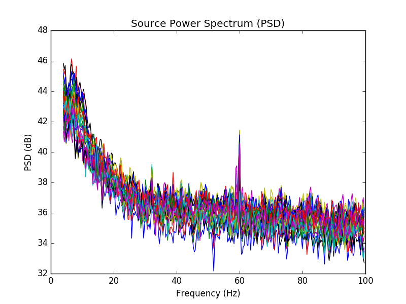
View PSD of sources in label
plt.plot(1e3 * stc.times, stc.data.T)
plt.xlabel('Frequency (Hz)')
plt.ylabel('PSD (dB)')
plt.title('Source Power Spectrum (PSD)')
plt.show()
Total running time of the script: ( 0 minutes 2.176 seconds)