Time-frequency on simulated data (Multitaper vs. Morlet)¶

# Authors: Hari Bharadwaj <hari@nmr.mgh.harvard.edu>
#          Denis Engemann <denis.engemann@gmail.com>
#
# License: BSD (3-clause)

import numpy as np

from mne import create_info, EpochsArray
from mne.time_frequency import tfr_multitaper, tfr_stockwell, tfr_morlet

print(__doc__)

sfreq = 1000.0
ch_names = ['SIM0001', 'SIM0002']
ch_types = ['grad', 'grad']
info = create_info(ch_names=ch_names, sfreq=sfreq, ch_types=ch_types)

n_times = int(sfreq)  # 1 second long epochs
n_epochs = 40
seed = 42
rng = np.random.RandomState(seed)
noise = rng.randn(n_epochs, len(ch_names), n_times)

# Add a 50 Hz sinusoidal burst to the noise and ramp it.
t = np.arange(n_times, dtype=np.float) / sfreq
signal = np.sin(np.pi * 2. * 50. * t)  # 50 Hz sinusoid signal
signal[np.logical_or(t < 0.45, t > 0.55)] = 0.  # Hard windowing
on_time = np.logical_and(t >= 0.45, t <= 0.55)
signal[on_time] *= np.hanning(on_time.sum())  # Ramping
data = noise + signal

reject = dict(grad=4000)
events = np.empty((n_epochs, 3), dtype=int)
first_event_sample = 100
event_id = dict(sin50hz=1)
for k in range(n_epochs):
    events[k, :] = first_event_sample + k * n_times, 0, event_id['sin50hz']

epochs = EpochsArray(data=data, info=info, events=events, event_id=event_id,
                     reject=reject)

freqs = np.arange(5., 100., 3.)

# You can trade time resolution or frequency resolution or both
# in order to get a reduction in variance

# (1) Least smoothing (most variance/background fluctuations).
n_cycles = freqs / 2.
time_bandwidth = 2.0  # Least possible frequency-smoothing (1 taper)
power = tfr_multitaper(epochs, freqs=freqs, n_cycles=n_cycles,
                       time_bandwidth=time_bandwidth, return_itc=False)
# Plot results. Baseline correct based on first 100 ms.
power.plot([0], baseline=(0., 0.1), mode='mean', vmin=-1., vmax=3.,
           title='Sim: Least smoothing, most variance')


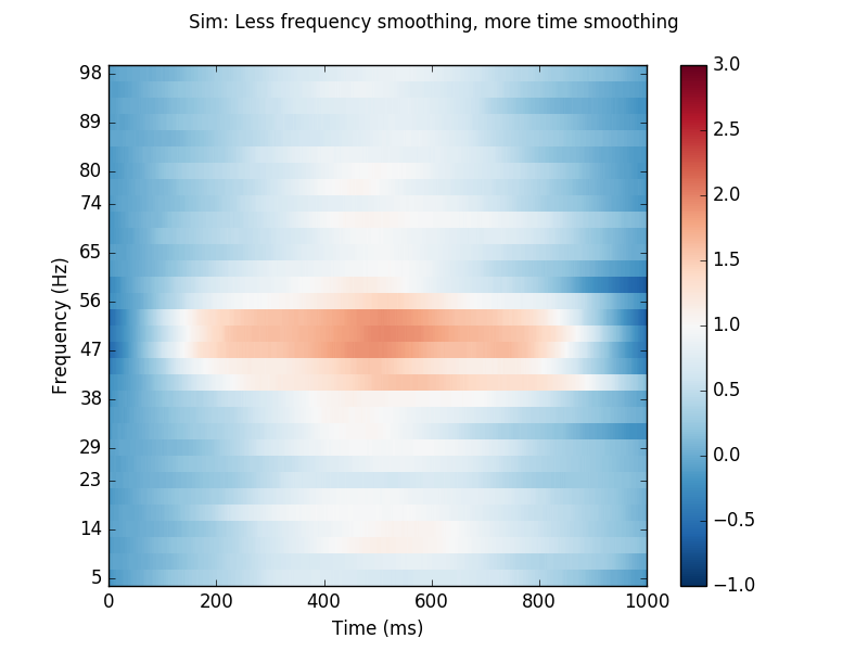
# (2) Less frequency smoothing, more time smoothing.
n_cycles = freqs  # Increase time-window length to 1 second.
time_bandwidth = 4.0  # Same frequency-smoothing as (1) 3 tapers.
power = tfr_multitaper(epochs, freqs=freqs, n_cycles=n_cycles,
                       time_bandwidth=time_bandwidth, return_itc=False)
# Plot results. Baseline correct based on first 100 ms.
power.plot([0], baseline=(0., 0.1), mode='mean', vmin=-1., vmax=3.,
           title='Sim: Less frequency smoothing, more time smoothing')


# (3) Less time smoothing, more frequency smoothing.
n_cycles = freqs / 2.
time_bandwidth = 8.0  # Same time-smoothing as (1), 7 tapers.
power = tfr_multitaper(epochs, freqs=freqs, n_cycles=n_cycles,
                       time_bandwidth=time_bandwidth, return_itc=False)
# Plot results. Baseline correct based on first 100 ms.
power.plot([0], baseline=(0., 0.1), mode='mean', vmin=-1., vmax=3.,
           title='Sim: Less time smoothing, more frequency smoothing')

# #############################################################################
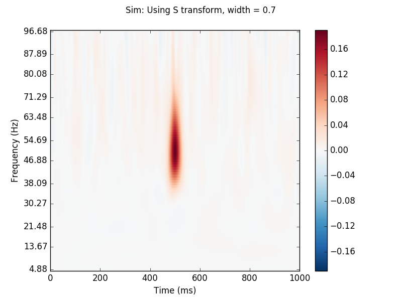
# Stockwell (S) transform

# S uses a Gaussian window to balance temporal and spectral resolution
# Importantly, frequency bands are phase-normalized, hence strictly comparable
# with regard to timing, and, the input signal can be recoverd from the
# transform in a lossless way if we disregard numerical errors.

fmin, fmax = freqs[[0, -1]]
for width in (0.7, 3.0):
    power = tfr_stockwell(epochs, fmin=fmin, fmax=fmax, width=width)
    power.plot([0], baseline=(0., 0.1), mode='mean',
               title='Sim: Using S transform, width '
                     '= {:0.1f}'.format(width), show=True)

# #############################################################################
# Finally, compare to morlet wavelet

n_cycles = freqs / 2.
power = tfr_morlet(epochs, freqs=freqs, n_cycles=n_cycles, return_itc=False)
power.plot([0], baseline=(0., 0.1), mode='mean', vmin=-1., vmax=3.,
           title='Sim: Using Morlet wavelet')