Some artifacts are restricted to certain frequencies and can therefore be fixed by filtering. An artifact that typically affects only some frequencies is due to the power line.
Power-line noise is a noise created by the electrical network. It is composed of sharp peaks at 50Hz (or 60Hz depending on your geographical location). Some peaks may also be present at the harmonic frequencies, i.e. the integer multiples of the power-line frequency, e.g. 100Hz, 150Hz, … (or 120Hz, 180Hz, …).
This tutorial covers some basics of how to filter data in MNE-Python. For more in-depth information about filter design in general and in MNE-Python in particular, check out Background information on filtering.
import numpy as np
import mne
from mne.datasets import sample
data_path = sample.data_path()
raw_fname = data_path + '/MEG/sample/sample_audvis_raw.fif'
proj_fname = data_path + '/MEG/sample/sample_audvis_eog_proj.fif'
tmin, tmax = 0, 20 # use the first 20s of data
# Setup for reading the raw data (save memory by cropping the raw data
# before loading it)
raw = mne.io.read_raw_fif(raw_fname)
raw.crop(tmin, tmax).load_data()
raw.info['bads'] = ['MEG 2443', 'EEG 053'] # bads + 2 more
fmin, fmax = 2, 300 # look at frequencies between 2 and 300Hz
n_fft = 2048 # the FFT size (n_fft). Ideally a power of 2
# Pick a subset of channels (here for speed reason)
selection = mne.read_selection('Left-temporal')
picks = mne.pick_types(raw.info, meg='mag', eeg=False, eog=False,
stim=False, exclude='bads', selection=selection)
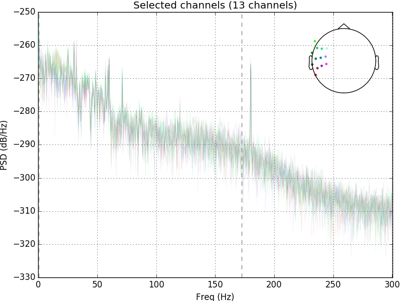
# Let's first check out all channel types
raw.plot_psd(area_mode='range', tmax=10.0, picks=picks, average=False)
Out:
Opening raw data file /home/ubuntu/mne_data/MNE-sample-data/MEG/sample/sample_audvis_raw.fif...
    Read a total of 3 projection items:
        PCA-v1 (1 x 10²)  idle
        PCA-v2 (1 x 10²)  idle
        PCA-v3 (1 x 10²)  idle
    Range : 25800 ... 192599 =     42.956 ...   320.670 secs
Ready.
Current compensation grade : 0
Reading 0 ... 12012  =      0.000 ...    20.000 secs...
Effective window size : 3.410 (s)
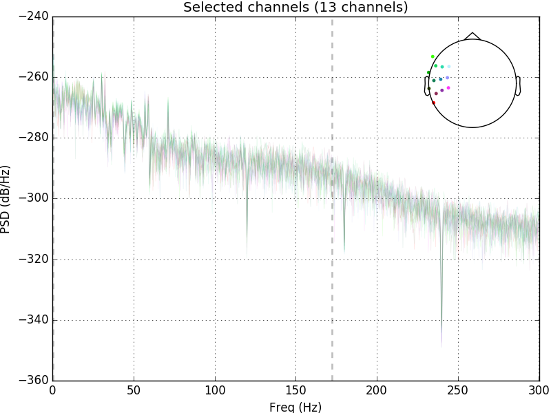
Removing power-line noise can be done with a Notch filter, directly on the Raw object, specifying an array of frequency to be cut off:
raw.notch_filter(np.arange(60, 241, 60), picks=picks, filter_length='auto',
                 phase='zero')
raw.plot_psd(area_mode='range', tmax=10.0, picks=picks, average=False)
Out:
Setting up band-stop filter
Filter length of 7928 samples (13.200 sec) selected
Effective window size : 3.410 (s)
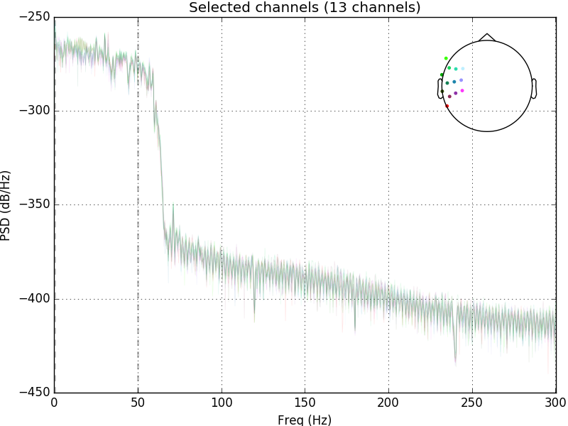
If you’re only interested in low frequencies, below the peaks of power-line noise you can simply low pass filter the data.
# low pass filtering below 50 Hz
raw.filter(None, 50., h_trans_bandwidth='auto', filter_length='auto',
           phase='zero')
raw.plot_psd(area_mode='range', tmax=10.0, picks=picks, average=False)
Out:
Setting up low-pass filter at 50 Hz
h_trans_bandwidth chosen to be 12.5 Hz
Filter length of 317 samples (0.528 sec) selected
Effective window size : 3.410 (s)
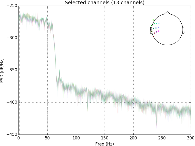
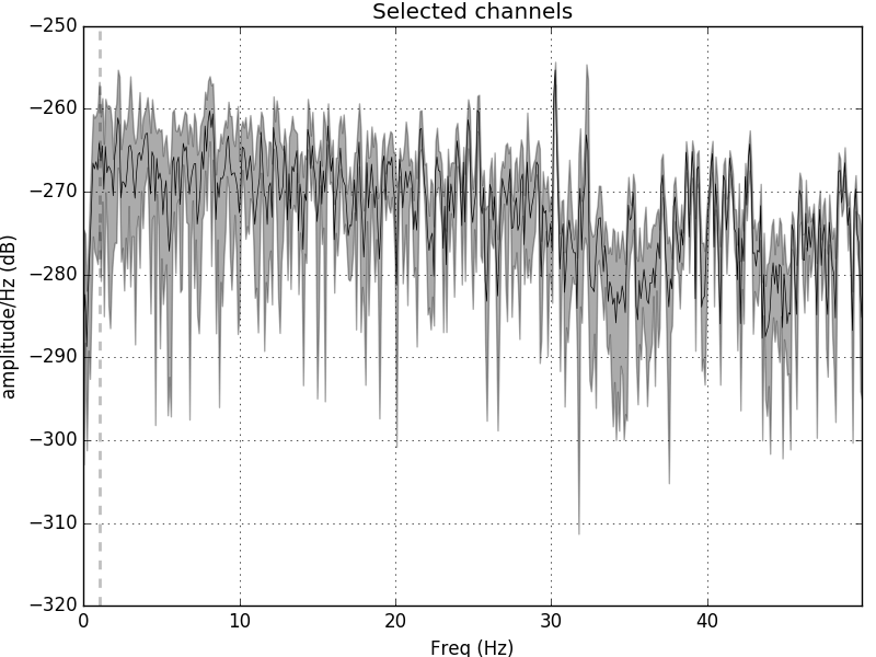
To remove slow drifts, you can high pass.
Warning
There can be issues using high-passes greater than 0.1 Hz (see examples in High-pass problems), so apply high-pass filters with caution.
raw.filter(1., None, l_trans_bandwidth='auto', filter_length='auto',
           phase='zero')
raw.plot_psd(area_mode='range', tmax=10.0, picks=picks, average=False)
Out:
Setting up high-pass filter at 1 Hz
l_trans_bandwidth chosen to be 1.0 Hz
Filter length of 3964 samples (6.600 sec) selected
Effective window size : 3.410 (s)
To do the low-pass and high-pass filtering in one step you can do a so-called band-pass filter by running the following:
# band-pass filtering in the range 1 Hz - 50 Hz
raw.filter(1, 50., l_trans_bandwidth='auto', h_trans_bandwidth='auto',
           filter_length='auto', phase='zero')
Out:
Setting up band-pass filter from 1 - 50 Hz
l_trans_bandwidth chosen to be 1.0 Hz
h_trans_bandwidth chosen to be 12.5 Hz
Filter length of 3964 samples (6.600 sec) selected
When performing experiments where timing is critical, a signal with a high sampling rate is desired. However, having a signal with a much higher sampling rate than necessary needlessly consumes memory and slows down computations operating on the data. To avoid that, you can downsample your time series. Since downsampling raw data reduces the timing precision of events, it is recommended only for use in procedures that do not require optimal precision, e.g. computing EOG or ECG projectors on long recordings.
Note
A downsampling operation performs a low-pass (to prevent
aliasing) followed by decimation, which selects every
\(N^{th}\) sample from the signal. See
scipy.signal.resample() and
scipy.signal.resample_poly() for examples.
Data resampling can be done with resample methods.
raw.resample(100, npad="auto")  # set sampling frequency to 100Hz
raw.plot_psd(area_mode='range', tmax=10.0, picks=picks)
Out:
25 events found
Events id: [ 1  2  3  4  5 32]
25 events found
Events id: [ 1  2  3  4  5 32]
Effective window size : 10.010 (s)
To avoid this reduction in precision, the suggested pipeline for processing final data to be analyzed is:
- low-pass the data with
mne.io.Raw.filter().- Extract epochs with
mne.Epochs.- Decimate the Epochs object using
mne.Epochs.decimate()or thedecimargument to themne.Epochsobject.
We also provide the convenience methods mne.Epochs.resample() and
mne.Evoked.resample() to downsample or upsample data, but these are
less optimal because they will introduce edge artifacts into every epoch,
whereas filtering the raw data will only introduce edge artifacts only at
the start and end of the recording.
Total running time of the script: ( 0 minutes 3.065 seconds)