Here we compute the evoked from raw for the Brainstorm Elekta phantom tutorial dataset. For comparison, see [1] and:
| [1] | Tadel F, Baillet S, Mosher JC, Pantazis D, Leahy RM. Brainstorm: A User-Friendly Application for MEG/EEG Analysis. Computational Intelligence and Neuroscience, vol. 2011, Article ID 879716, 13 pages, 2011. doi:10.1155/2011/879716 |
# Authors: Eric Larson <larson.eric.d@gmail.com>
#
# License: BSD (3-clause)

import os.path as op
import numpy as np

import mne
from mne import find_events, fit_dipole
from mne.datasets.brainstorm import bst_phantom_elekta
from mne.io import read_raw_fif

print(__doc__)
The data were collected with an Elekta Neuromag VectorView system at 1000 Hz
and low-pass filtered at 330 Hz. Here the medium-amplitude (200 nAm) data
are read to construct instances of mne.io.Raw.
data_path = bst_phantom_elekta.data_path()

raw_fname = op.join(data_path, 'kojak_all_200nAm_pp_no_chpi_no_ms_raw.fif')
raw = read_raw_fif(raw_fname)
Out:
Opening raw data file /home/ubuntu/mne_data/MNE-brainstorm-data/bst_phantom_elekta/kojak_all_200nAm_pp_no_chpi_no_ms_raw.fif...
    Read a total of 13 projection items:
        planar-0.0-115.0-PCA-01 (1 x 306)  idle
        planar-0.0-115.0-PCA-02 (1 x 306)  idle
        planar-0.0-115.0-PCA-03 (1 x 306)  idle
        planar-0.0-115.0-PCA-04 (1 x 306)  idle
        planar-0.0-115.0-PCA-05 (1 x 306)  idle
        axial-0.0-115.0-PCA-01 (1 x 306)  idle
        axial-0.0-115.0-PCA-02 (1 x 306)  idle
        axial-0.0-115.0-PCA-03 (1 x 306)  idle
        axial-0.0-115.0-PCA-04 (1 x 306)  idle
        axial-0.0-115.0-PCA-05 (1 x 306)  idle
        axial-0.0-115.0-PCA-06 (1 x 306)  idle
        axial-0.0-115.0-PCA-07 (1 x 306)  idle
        axial-0.0-115.0-PCA-08 (1 x 306)  idle
    Range : 47000 ... 437999 =     47.000 ...   437.999 secs
Ready.
Current compensation grade : 0
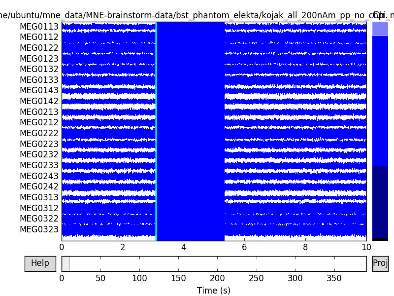
Data channel array consisted of 204 MEG planor gradiometers, 102 axial magnetometers, and 3 stimulus channels. Let’s get the events for the phantom, where each dipole (1-32) gets its own event:
events = find_events(raw, 'STI201')
raw.plot(events=events)
raw.info['bads'] = ['MEG2421']
Out:
645 events found
Events id: [   1    2    3    4    5    6    7    8    9   10   11   12   13   14   15
   16   17   18   19   20   21   22   23   24   25   26   27   28   29   30
   31   32  256  768 1792 3840 7936]
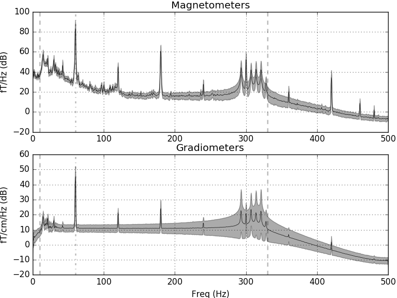
The data have strong line frequency (60 Hz and harmonics) and cHPI coil noise (five peaks around 300 Hz). Here we plot only out to 60 seconds to save memory:
raw.plot_psd(tmax=60.)
Out:
Effective window size : 2.048 (s)
Effective window size : 2.048 (s)
Let’s use Maxwell filtering to clean the data a bit. Ideally we would have the fine calibration and cross-talk information for the site of interest, but we don’t, so we just do:
raw.fix_mag_coil_types()
raw = mne.preprocessing.maxwell_filter(raw, origin=(0., 0., 0.))
Out:
101 of 101 T1/T2 magnetometer types replaced with T3.
Maxwell filtering raw data
    Loading raw data from disk
    Bad MEG channels being reconstructed: ['MEG2421']
    Processing 204 gradiometers and 102 magnetometers
    Using origin 0.0, 0.0, 0.0 mm in the head frame
    Computing regularization
        Using 87/95 harmonic components for    0.000  (72/80 in, 15/15 out)
    Processing 39 data chunks of (at least) 10.0 sec
[done]
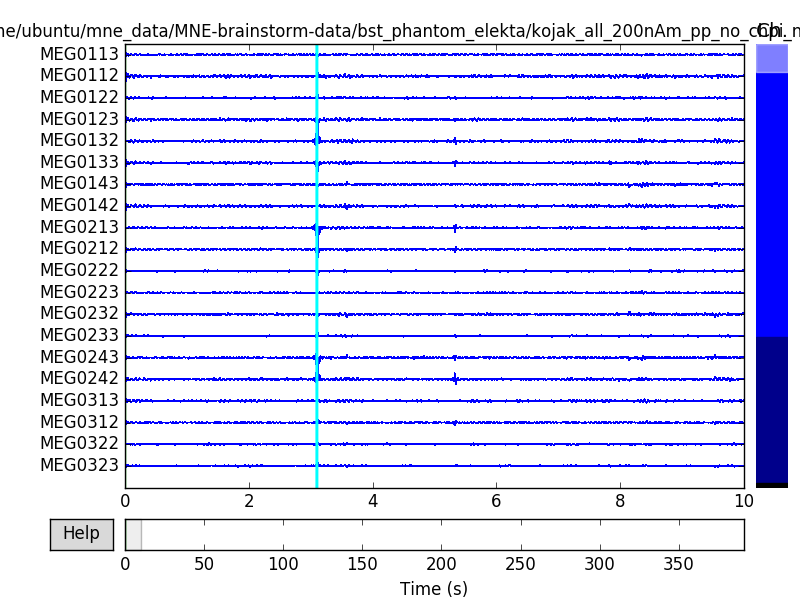
We know our phantom produces sinusoidal bursts below 25 Hz, so let’s filter.
raw.filter(None, 40., h_trans_bandwidth='auto', filter_length='auto',
           phase='zero', fir_window='hamming')
raw.plot(events=events)
Out:
Setting up low-pass filter at 40 Hz
h_trans_bandwidth chosen to be 10.0 Hz
Filter length of 660 samples (0.660 sec) selected
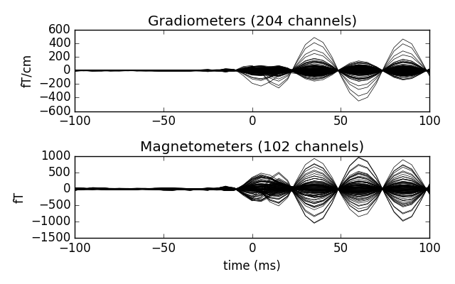
Now we epoch our data, average it, and look at the first dipole response. The first peak appears around 3 ms. Because we low-passed at 40 Hz, we can also decimate our data to save memory.
tmin, tmax = -0.1, 0.1
event_id = list(range(1, 33))
epochs = mne.Epochs(raw, events, event_id, tmin, tmax, baseline=(None, -0.01),
                    decim=5, preload=True)
epochs['1'].average().plot()
Out:
640 matching events found
0 projection items activated
Loading data for 640 events and 201 original time points ...
0 bad epochs dropped
Let’s do some dipole fits. The phantom is properly modeled by a single-shell sphere with origin (0., 0., 0.). We compute covariance, then do the fits.
t_peak = 60e-3  # ~60 MS at largest peak
sphere = mne.make_sphere_model(r0=(0., 0., 0.), head_radius=None)
cov = mne.compute_covariance(epochs, tmax=0)
data = []
for ii in range(1, 33):
    evoked = epochs[str(ii)].average().crop(t_peak, t_peak)
    data.append(evoked.data[:, 0])
evoked = mne.EvokedArray(np.array(data).T, evoked.info, tmin=0.)
del epochs, raw
dip = fit_dipole(evoked, cov, sphere, n_jobs=1)[0]
Out:
Estimating covariance using EMPIRICAL
Done.
Using cross-validation to select the best estimator.
Number of samples used : 13440
[done]
log-likelihood on unseen data (descending order):
   empirical: -4741.686
selecting best estimator: empirical
BEM               : <ConductorModel  |  Sphere (no layers): r0=[0.0, 0.0, 0.0] mm>
Sphere model      : origin at (   0.00    0.00    0.00) mm, max_rad =    0.1 mm
Guess grid        :   20.0 mm
Guess mindist     :    5.0 mm
Guess exclude     :   20.0 mm
Using standard MEG coil definitions.

Coordinate transformation: head -> MRI (surface RAS)
     1.000000  0.000000  0.000000       0.00 mm
     0.000000  1.000000  0.000000       0.00 mm
     0.000000  0.000000  1.000000       0.00 mm
     0.000000  0.000000  0.000000       1.00
Coordinate transformation: MEG device -> head
     0.976295 -0.211976  0.043756       0.29 mm
     0.206488  0.972764  0.105326       0.57 mm
    -0.064891 -0.093794  0.993475       5.41 mm
     0.000000  0.000000  0.000000       1.00
0 bad channels total
Read 306 MEG channels from info
81 coil definitions read
Coordinate transformation: MEG device -> head
     0.976295 -0.211976  0.043756       0.29 mm
     0.206488  0.972764  0.105326       0.57 mm
    -0.064891 -0.093794  0.993475       5.41 mm
     0.000000  0.000000  0.000000       1.00
MEG coil definitions created in head coordinates.
Decomposing the sensor noise covariance matrix...

---- Computing the forward solution for the guesses...
Making a spherical guess space with radius   107.7 mm...
Filtering (grid =     20 mm)...
Surface CM = (   0.0   -0.0    0.0) mm
Surface fits inside a sphere with radius  107.7 mm
Surface extent:
    x = -107.7 ...  107.7 mm
    y = -107.7 ...  107.7 mm
    z = -107.7 ...  107.7 mm
Grid extent:
    x = -120.0 ...  120.0 mm
    y = -120.0 ...  120.0 mm
    z = -120.0 ...  120.0 mm
2197 sources before omitting any.
687 sources after omitting infeasible sources.
Source spaces are in MRI coordinates.
Checking that the sources are inside the bounding surface and at least    5.0 mm away (will take a few...)
72 source space points omitted because they are outside the inner skull surface.
4 source space points omitted because of the    5.0-mm distance limit.
Thank you for waiting.
611 sources remaining after excluding the sources outside the surface and less than    5.0 mm inside.
Go through all guess source locations...
[done 611 sources]
---- Fitted :     0.0 ms
---- Fitted :     5.0 ms
---- Fitted :    10.0 ms
---- Fitted :    15.0 ms
---- Fitted :    20.0 ms
---- Fitted :    25.0 ms
---- Fitted :    30.0 ms
---- Fitted :    35.0 ms
---- Fitted :    40.0 ms
---- Fitted :    45.0 ms
---- Fitted :    50.0 ms
---- Fitted :    55.0 ms
---- Fitted :    60.0 ms
---- Fitted :    65.0 ms
---- Fitted :    70.0 ms
---- Fitted :    75.0 ms
---- Fitted :    80.0 ms
---- Fitted :    85.0 ms
---- Fitted :    90.0 ms
---- Fitted :    95.0 ms
---- Fitted :   100.0 ms
---- Fitted :   105.0 ms
---- Fitted :   110.0 ms
---- Fitted :   115.0 ms
---- Fitted :   120.0 ms
---- Fitted :   125.0 ms
---- Fitted :   130.0 ms
---- Fitted :   135.0 ms
---- Fitted :   140.0 ms
---- Fitted :   145.0 ms
---- Fitted :   150.0 ms
---- Fitted :   155.0 ms
32 time points fitted
Now we can compare to the actual locations, taking the difference in mm:
actual_pos = mne.dipole.get_phantom_dipoles()[0]
diffs = 1000 * np.sqrt(np.sum((dip.pos - actual_pos) ** 2, axis=-1))
print('Differences (mm):\n%s' % diffs[:, np.newaxis])
print('μ = %s' % (np.mean(diffs),))
Out:
Differences (mm):
[[ 1.71653987]
 [ 1.78034826]
 [ 2.41151691]
 [ 2.25981748]
 [ 2.35041079]
 [ 2.26054589]
 [ 3.11698303]
 [ 1.35122427]
 [ 1.75220455]
 [ 1.64285627]
 [ 1.04087526]
 [ 1.54661897]
 [ 2.50100245]
 [ 2.51564406]
 [ 1.56668003]
 [ 2.08579421]
 [ 2.72381663]
 [ 2.44380679]
 [ 2.42802786]
 [ 1.31589791]
 [ 1.84485872]
 [ 2.10459702]
 [ 2.50569254]
 [ 1.15682919]
 [ 2.10908197]
 [ 2.2329816 ]
 [ 1.38032152]
 [ 1.40415623]
 [ 2.78747421]
 [ 2.16451656]
 [ 1.33393775]
 [ 4.13154386]]
μ = 2.06145633345
Total running time of the script: ( 0 minutes 29.555 seconds)