MNE supports working with more than just MEG and EEG data. Here we show some of the functions that can be used to facilitate working with electrocorticography (ECoG) data.
# Authors: Eric Larson <larson.eric.d@gmail.com>
#          Chris Holdgraf <choldgraf@gmail.com>
#
# License: BSD (3-clause)

import numpy as np
import matplotlib.pyplot as plt
from scipy.io import loadmat
from mayavi import mlab

import mne
from mne.viz import plot_trans, snapshot_brain_montage

print(__doc__)
Let’s load some ECoG electrode locations and names, and turn them into
a mne.channels.DigMontage class.
mat = loadmat(mne.datasets.misc.data_path() + '/ecog/sample_ecog.mat')
ch_names = mat['ch_names'].tolist()
elec = mat['elec']
dig_ch_pos = dict(zip(ch_names, elec))
mon = mne.channels.DigMontage(dig_ch_pos=dig_ch_pos)
print('Created %s channel positions' % len(ch_names))
Out:
Created 64 channel positions
Now that we have our electrode positions in MRI coordinates, we can create our measurement info structure.
info = mne.create_info(ch_names, 1000., 'ecog', montage=mon)
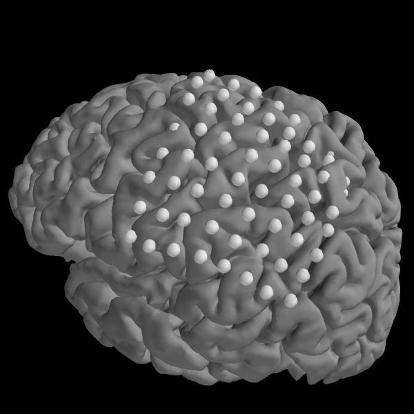
We can then plot the locations of our electrodes on our subject’s brain.
Note
These are not real electrodes for this subject, so they do not align to the cortical surface perfectly.
subjects_dir = mne.datasets.sample.data_path() + '/subjects'
fig = plot_trans(info, trans=None, subject='sample', subjects_dir=subjects_dir)
mlab.view(200, 70)
Out:
MEG electrodes not found. Cannot plot MEG locations.
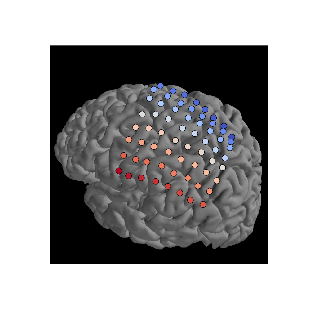
Sometimes it is useful to make a scatterplot for the current figure view. This is best accomplished with matplotlib. We can capture an image of the current mayavi view, along with the xy position of each electrode, with the snapshot_brain_montage function.
# We'll once again plot the surface, then take a snapshot.
fig = plot_trans(info, trans=None, subject='sample', subjects_dir=subjects_dir)
mlab.view(200, 70)
xy, im = snapshot_brain_montage(fig, mon)

# Convert from a dictionary to array to plot
xy_pts = np.vstack(xy[ch] for ch in info['ch_names'])

# Define an arbitrary "activity" pattern for viz
activity = np.linspace(100, 200, xy_pts.shape[0])

# This allows us to use matplotlib to create arbitrary 2d scatterplots
_, ax = plt.subplots(figsize=(10, 10))
ax.imshow(im)
ax.scatter(*xy_pts.T, c=activity, s=200, cmap='coolwarm')
ax.set_axis_off()
plt.show()

Out:
MEG electrodes not found. Cannot plot MEG locations.
Total running time of the script: ( 0 minutes 15.350 seconds)