from __future__ import print_function

import mne
import os.path as op
import numpy as np
from matplotlib import pyplot as plt
It is often necessary to modify data once you have loaded it into memory. Common examples of this are signal processing, feature extraction, and data cleaning. Some functionality is pre-built into MNE-python, though it is also possible to apply an arbitrary function to the data.
# Load an example dataset, the preload flag loads the data into memory now
data_path = op.join(mne.datasets.sample.data_path(), 'MEG',
                    'sample', 'sample_audvis_raw.fif')
raw = mne.io.read_raw_fif(data_path, preload=True)
raw = raw.crop(0, 10)
print(raw)
Out:
Opening raw data file /home/ubuntu/mne_data/MNE-sample-data/MEG/sample/sample_audvis_raw.fif...
    Read a total of 3 projection items:
        PCA-v1 (1 x 10²)  idle
        PCA-v2 (1 x 10²)  idle
        PCA-v3 (1 x 10²)  idle
    Range : 25800 ... 192599 =     42.956 ...   320.670 secs
Ready.
Current compensation grade : 0
Reading 0 ... 166799  =      0.000 ...   277.714 secs...
<Raw  |  sample_audvis_raw.fif, n_channels x n_times : 376 x 6007 (10.0 sec), ~21.0 MB, data loaded>
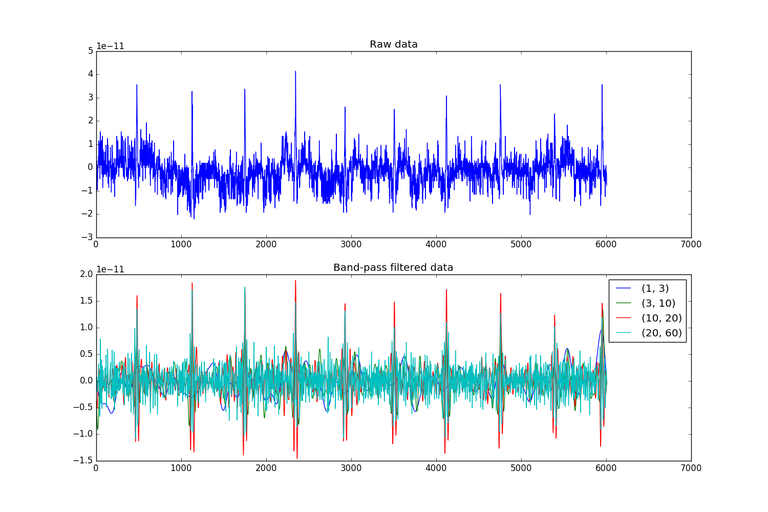
Most MNE objects have in-built methods for filtering:
filt_bands = [(1, 3), (3, 10), (10, 20), (20, 60)]
f, (ax, ax2) = plt.subplots(2, 1, figsize=(15, 10))
_ = ax.plot(raw._data[0])
for fband in filt_bands:
    raw_filt = raw.copy()
    raw_filt.filter(*fband, h_trans_bandwidth='auto', l_trans_bandwidth='auto',
                    filter_length='auto', phase='zero')
    _ = ax2.plot(raw_filt[0][0][0])
ax2.legend(filt_bands)
ax.set_title('Raw data')
ax2.set_title('Band-pass filtered data')
Out:
Setting up band-pass filter from 1 - 3 Hz
l_trans_bandwidth chosen to be 1.0 Hz
h_trans_bandwidth chosen to be 2.0 Hz
Filter length of 3964 samples (6.600 sec) selected
Setting up band-pass filter from 3 - 10 Hz
l_trans_bandwidth chosen to be 2.0 Hz
h_trans_bandwidth chosen to be 2.5 Hz
Filter length of 1982 samples (3.300 sec) selected
Setting up band-pass filter from 10 - 20 Hz
l_trans_bandwidth chosen to be 2.5 Hz
h_trans_bandwidth chosen to be 5.0 Hz
Filter length of 1586 samples (2.641 sec) selected
Setting up band-pass filter from 20 - 60 Hz
l_trans_bandwidth chosen to be 5.0 Hz
h_trans_bandwidth chosen to be 15.0 Hz
Filter length of 793 samples (1.320 sec) selected
In addition, there are functions for applying the Hilbert transform, which is useful to calculate phase / amplitude of your signal.
# Filter signal with a fairly steep filter, then take hilbert transform

raw_band = raw.copy()
raw_band.filter(12, 18, l_trans_bandwidth=2., h_trans_bandwidth=2.,
                filter_length='auto', phase='zero')
raw_hilb = raw_band.copy()
hilb_picks = mne.pick_types(raw_band.info, meg=False, eeg=True)
raw_hilb.apply_hilbert(hilb_picks)
print(raw_hilb._data.dtype)
Out:
Setting up band-pass filter from 12 - 18 Hz
Filter length of 1982 samples (3.300 sec) selected
complex64
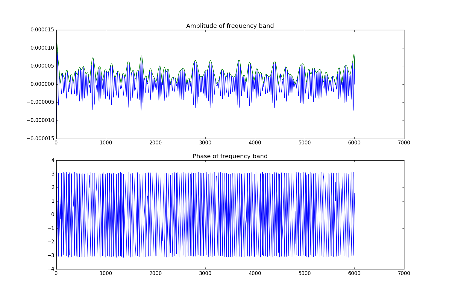
Finally, it is possible to apply arbitrary functions to your data to do what you want. Here we will use this to take the amplitude and phase of the hilbert transformed data.
Note
You can also use amplitude=True in the call to
mne.io.Raw.apply_hilbert() to do this automatically.
# Take the amplitude and phase
raw_amp = raw_hilb.copy()
raw_amp.apply_function(np.abs, hilb_picks)
raw_phase = raw_hilb.copy()
raw_phase.apply_function(np.angle, hilb_picks)

f, (a1, a2) = plt.subplots(2, 1, figsize=(15, 10))
a1.plot(raw_band._data[hilb_picks[0]])
a1.plot(raw_amp._data[hilb_picks[0]])
a2.plot(raw_phase._data[hilb_picks[0]])
a1.set_title('Amplitude of frequency band')
a2.set_title('Phase of frequency band')
Total running time of the script: ( 0 minutes 2.901 seconds)