![]()
The aim of this tutorial is to demonstrate how to put a known signal at a
desired location(s) in a mne.SourceEstimate and then corrupt the
signal with point-spread by applying a forward and inverse solution.
import os.path as op

import numpy as np
from mayavi import mlab

import mne
from mne.datasets import sample

from mne.minimum_norm import read_inverse_operator, apply_inverse
from mne.simulation import simulate_stc, simulate_evoked
First, we set some parameters.
seed = 42

# parameters for inverse method
method = 'sLORETA'
snr = 3.
lambda2 = 1.0 / snr ** 2

# signal simulation parameters
# do not add extra noise to the known signals
evoked_snr = np.inf
T = 100
times = np.linspace(0, 1, T)
dt = times[1] - times[0]

# Paths to MEG data
data_path = sample.data_path()
subjects_dir = op.join(data_path, 'subjects')
fname_fwd = op.join(data_path, 'MEG', 'sample',
                    'sample_audvis-meg-oct-6-fwd.fif')
fname_inv = op.join(data_path, 'MEG', 'sample',
                    'sample_audvis-meg-oct-6-meg-fixed-inv.fif')

fname_evoked = op.join(data_path, 'MEG', 'sample',
                       'sample_audvis-ave.fif')
fwd = mne.read_forward_solution(fname_fwd, force_fixed=True,
                                surf_ori=True)
fwd['info']['bads'] = []
inv_op = read_inverse_operator(fname_inv)

raw = mne.io.RawFIF(op.join(data_path, 'MEG', 'sample',
                            'sample_audvis_raw.fif'))
events = mne.find_events(raw)
event_id = {'Auditory/Left': 1, 'Auditory/Right': 2}
epochs = mne.Epochs(raw, events, event_id, baseline=(None, 0), preload=True)
epochs.info['bads'] = []
evoked = epochs.average()

labels = mne.read_labels_from_annot('sample', subjects_dir=subjects_dir)
label_names = [l.name for l in labels]
n_labels = len(labels)
Out:
Reading forward solution from /home/ubuntu/mne_data/MNE-sample-data/MEG/sample/sample_audvis-meg-oct-6-fwd.fif...
    Reading a source space...
    Computing patch statistics...
    Patch information added...
    Distance information added...
    [done]
    Reading a source space...
    Computing patch statistics...
    Patch information added...
    Distance information added...
    [done]
    2 source spaces read
    Desired named matrix (kind = 3523) not available
    Read MEG forward solution (7498 sources, 306 channels, free orientations)
    Source spaces transformed to the forward solution coordinate frame
    Changing to fixed-orientation forward solution with surface-based source orientations...
    [done]
Reading inverse operator decomposition from /home/ubuntu/mne_data/MNE-sample-data/MEG/sample/sample_audvis-meg-oct-6-meg-fixed-inv.fif...
    Reading inverse operator info...
    [done]
    Reading inverse operator decomposition...
    [done]
    305 x 305 full covariance (kind = 1) found.
    Read a total of 4 projection items:
        PCA-v1 (1 x 10²) active
        PCA-v2 (1 x 10²) active
        PCA-v3 (1 x 10²) active
        Average EEG reference (1 x 60) active
    Noise covariance matrix read.
    7498 x 7498 diagonal covariance (kind = 2) found.
    Source covariance matrix read.
    Did not find the desired covariance matrix (kind = 6)
    7498 x 7498 diagonal covariance (kind = 5) found.
    Depth priors read.
    Did not find the desired covariance matrix (kind = 3)
    Reading a source space...
    Computing patch statistics...
    Patch information added...
    Distance information added...
    [done]
    Reading a source space...
    Computing patch statistics...
    Patch information added...
    Distance information added...
    [done]
    2 source spaces read
    Read a total of 4 projection items:
        PCA-v1 (1 x 10²) active
        PCA-v2 (1 x 10²) active
        PCA-v3 (1 x 10²) active
        Average EEG reference (1 x 60) active
    Source spaces transformed to the inverse solution coordinate frame
Opening raw data file /home/ubuntu/mne_data/MNE-sample-data/MEG/sample/sample_audvis_raw.fif...
    Read a total of 3 projection items:
        PCA-v1 (1 x 10²)  idle
        PCA-v2 (1 x 10²)  idle
        PCA-v3 (1 x 10²)  idle
    Range : 25800 ... 192599 =     42.956 ...   320.670 secs
Ready.
Current compensation grade : 0
320 events found
Events id: [ 1  2  3  4  5 32]
145 matching events found
Created an SSP operator (subspace dimension = 3)
3 projection items activated
Loading data for 145 events and 421 original time points ...
0 bad epochs dropped
Reading labels from parcellation..
   read 34 labels from /home/ubuntu/mne_data/MNE-sample-data/subjects/sample/label/lh.aparc.annot
   read 34 labels from /home/ubuntu/mne_data/MNE-sample-data/subjects/sample/label/rh.aparc.annot
[done]
cov = mne.compute_covariance(epochs, tmin=None, tmax=0.)
Out:
Estimating covariance using EMPIRICAL
Done.
Using cross-validation to select the best estimator.
Number of samples used : 17545
[done]
log-likelihood on unseen data (descending order):
   empirical: -1814.827
selecting best estimator: empirical
# The known signal is all zero-s off of the two labels of interest
signal = np.zeros((n_labels, T))
idx = label_names.index('inferiorparietal-lh')
signal[idx, :] = 1e-7 * np.sin(5 * 2 * np.pi * times)
idx = label_names.index('rostralmiddlefrontal-rh')
signal[idx, :] = 1e-7 * np.sin(7 * 2 * np.pi * times)
We want the known signal in each label to only be active at the center. We create a mask for each label that is 1 at the center vertex and 0 at all other vertices in the label. This mask is then used when simulating source-space data.
hemi_to_ind = {'lh': 0, 'rh': 1}
for i, label in enumerate(labels):
    # The `center_of_mass` function needs labels to have values.
    labels[i].values.fill(1.)

    # Restrict the eligible vertices to be those on the surface under
    # consideration and within the label.
    surf_vertices = fwd['src'][hemi_to_ind[label.hemi]]['vertno']
    restrict_verts = np.intersect1d(surf_vertices, label.vertices)
    com = labels[i].center_of_mass(subject='sample',
                                   subjects_dir=subjects_dir,
                                   restrict_vertices=restrict_verts,
                                   surf='white')

    # Convert the center of vertex index from surface vertex list to Label's
    # vertex list.
    cent_idx = np.where(label.vertices == com)[0][0]

    # Create a mask with 1 at center vertex and zeros elsewhere.
    labels[i].values.fill(0.)
    labels[i].values[cent_idx] = 1.
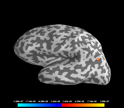
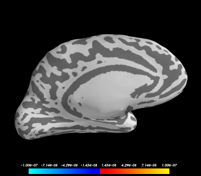
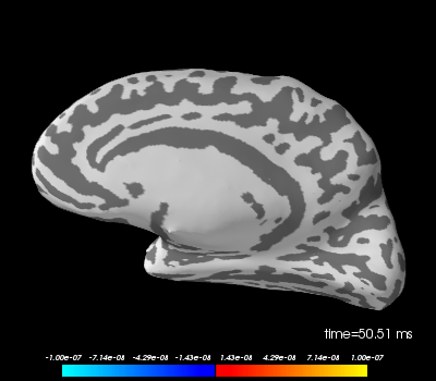
Put known signals onto surface vertices using the array of signals and the label masks (stored in labels[i].values).
stc_gen = simulate_stc(fwd['src'], labels, signal, times[0], dt,
                       value_fun=lambda x: x)
Note that the original signals are highly concentrated (point) sources.
kwargs = dict(subjects_dir=subjects_dir, hemi='split', smoothing_steps=4,
              time_unit='s', initial_time=0.05, size=1200,
              views=['lat', 'med'])
clim = dict(kind='value', pos_lims=[1e-9, 1e-8, 1e-7])
figs = [mlab.figure(1), mlab.figure(2), mlab.figure(3), mlab.figure(4)]
brain_gen = stc_gen.plot(clim=clim, figure=figs, **kwargs)

Out:
Updating smoothing matrix, be patient..
Smoothing matrix creation, step 1
Smoothing matrix creation, step 2
Smoothing matrix creation, step 3
Smoothing matrix creation, step 4
colormap: fmin=-1.00e-07 fmid=0.00e+00 fmax=1.00e-07 transparent=0
Updating smoothing matrix, be patient..
Smoothing matrix creation, step 1
Smoothing matrix creation, step 2
Smoothing matrix creation, step 3
Smoothing matrix creation, step 4
colormap: fmin=-1.00e-07 fmid=0.00e+00 fmax=1.00e-07 transparent=0
Use the forward solution and add Gaussian noise to simulate sensor-space (evoked) data from the known source-space signals. The amount of noise is controlled by evoked_snr (higher values imply less noise).
evoked_gen = simulate_evoked(fwd, stc_gen, evoked.info, cov, evoked_snr,
                             tmin=0., tmax=1., random_state=seed)

# Map the simulated sensor-space data to source-space using the inverse
# operator.
stc_inv = apply_inverse(evoked_gen, inv_op, lambda2, method=method)
Out:
Projecting source estimate to sensor space...
[done]
Preparing the inverse operator for use...
    Scaled noise and source covariance from nave = 1 to nave = 1
    Created the regularized inverter
    Created an SSP operator (subspace dimension = 3)
    Created the whitener using a full noise covariance matrix (3 small eigenvalues omitted)
    Computing noise-normalization factors (sLORETA)...
[done]
Picked 305 channels from the data
Computing inverse...
(eigenleads need to be weighted)...
(dSPM)...
[done]
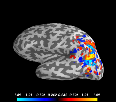
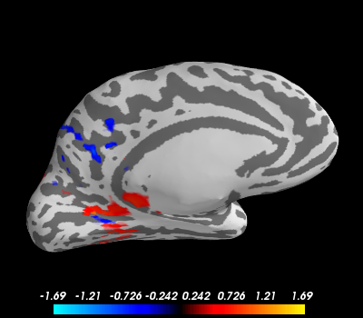
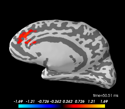
Notice that after applying the forward- and inverse-operators to the known point sources that the point sources have spread across the source-space. This spread is due to the minimum norm solution so that the signal leaks to nearby vertices with similar orientations so that signal ends up crossing the sulci and gyri.
figs = [mlab.figure(5), mlab.figure(6), mlab.figure(7), mlab.figure(8)]
brain_inv = stc_inv.plot(figure=figs, **kwargs)

Out:
Updating smoothing matrix, be patient..
Smoothing matrix creation, step 1
Smoothing matrix creation, step 2
Smoothing matrix creation, step 3
Smoothing matrix creation, step 4
colormap: fmin=-1.69e+00 fmid=0.00e+00 fmax=1.69e+00 transparent=0
Updating smoothing matrix, be patient..
Smoothing matrix creation, step 1
Smoothing matrix creation, step 2
Smoothing matrix creation, step 3
Smoothing matrix creation, step 4
colormap: fmin=-1.69e+00 fmid=0.00e+00 fmax=1.69e+00 transparent=0
- Change the method parameter to either dSPM or MNE to explore the effect of the inverse method.
- Try setting evoked_snr to a small, finite value, e.g. 3., to see the effect of noise.
Total running time of the script: ( 1 minutes 18.631 seconds)