Tests if the evoked response is significantly different between conditions across subjects (simulated here using one subject’s data). The multiple comparisons problem is addressed with a cluster-level permutation test across space and time.
# Authors: Alexandre Gramfort <alexandre.gramfort@telecom-paristech.fr>
#          Eric Larson <larson.eric.d@gmail.com>
# License: BSD (3-clause)


import os.path as op

import numpy as np
from numpy.random import randn
from scipy import stats as stats

import mne
from mne import (io, spatial_tris_connectivity, compute_morph_matrix,
                 grade_to_tris)
from mne.epochs import equalize_epoch_counts
from mne.stats import (spatio_temporal_cluster_1samp_test,
                       summarize_clusters_stc)
from mne.minimum_norm import apply_inverse, read_inverse_operator
from mne.datasets import sample

print(__doc__)
data_path = sample.data_path()
raw_fname = data_path + '/MEG/sample/sample_audvis_filt-0-40_raw.fif'
event_fname = data_path + '/MEG/sample/sample_audvis_filt-0-40_raw-eve.fif'
subjects_dir = data_path + '/subjects'

tmin = -0.2
tmax = 0.3  # Use a lower tmax to reduce multiple comparisons

#   Setup for reading the raw data
raw = io.read_raw_fif(raw_fname)
events = mne.read_events(event_fname)
Out:
Opening raw data file /home/ubuntu/mne_data/MNE-sample-data/MEG/sample/sample_audvis_filt-0-40_raw.fif...
    Read a total of 4 projection items:
        PCA-v1 (1 x 10²)  idle
        PCA-v2 (1 x 10²)  idle
        PCA-v3 (1 x 10²)  idle
        Average EEG reference (1 x 60)  idle
    Range : 6450 ... 48149 =     42.956 ...   320.665 secs
Ready.
Current compensation grade : 0
raw.info['bads'] += ['MEG 2443']
picks = mne.pick_types(raw.info, meg=True, eog=True, exclude='bads')
event_id = 1  # L auditory
reject = dict(grad=1000e-13, mag=4000e-15, eog=150e-6)
epochs1 = mne.Epochs(raw, events, event_id, tmin, tmax, picks=picks,
                     baseline=(None, 0), reject=reject, preload=True)

event_id = 3  # L visual
epochs2 = mne.Epochs(raw, events, event_id, tmin, tmax, picks=picks,
                     baseline=(None, 0), reject=reject, preload=True)

#    Equalize trial counts to eliminate bias (which would otherwise be
#    introduced by the abs() performed below)
equalize_epoch_counts([epochs1, epochs2])
Out:
72 matching events found
Created an SSP operator (subspace dimension = 3)
4 projection items activated
Loading data for 72 events and 76 original time points ...
    Rejecting  epoch based on EOG : [u'EOG 061']
    Rejecting  epoch based on EOG : [u'EOG 061']
    Rejecting  epoch based on EOG : [u'EOG 061']
    Rejecting  epoch based on EOG : [u'EOG 061']
    Rejecting  epoch based on MAG : [u'MEG 1711']
    Rejecting  epoch based on EOG : [u'EOG 061']
    Rejecting  epoch based on EOG : [u'EOG 061']
    Rejecting  epoch based on EOG : [u'EOG 061']
    Rejecting  epoch based on EOG : [u'EOG 061']
9 bad epochs dropped
73 matching events found
Created an SSP operator (subspace dimension = 3)
4 projection items activated
Loading data for 73 events and 76 original time points ...
    Rejecting  epoch based on EOG : [u'EOG 061']
    Rejecting  epoch based on EOG : [u'EOG 061']
    Rejecting  epoch based on EOG : [u'EOG 061']
    Rejecting  epoch based on EOG : [u'EOG 061']
    Rejecting  epoch based on GRAD : [u'MEG 1333', u'MEG 1342']
    Rejecting  epoch based on EOG : [u'EOG 061']
6 bad epochs dropped
Dropped 0 epochs
Dropped 4 epochs
fname_inv = data_path + '/MEG/sample/sample_audvis-meg-oct-6-meg-inv.fif'
snr = 3.0
lambda2 = 1.0 / snr ** 2
method = "dSPM"  # use dSPM method (could also be MNE or sLORETA)
inverse_operator = read_inverse_operator(fname_inv)
sample_vertices = [s['vertno'] for s in inverse_operator['src']]

#    Let's average and compute inverse, resampling to speed things up
evoked1 = epochs1.average()
evoked1.resample(50, npad='auto')
condition1 = apply_inverse(evoked1, inverse_operator, lambda2, method)
evoked2 = epochs2.average()
evoked2.resample(50, npad='auto')
condition2 = apply_inverse(evoked2, inverse_operator, lambda2, method)

#    Let's only deal with t > 0, cropping to reduce multiple comparisons
condition1.crop(0, None)
condition2.crop(0, None)
tmin = condition1.tmin
tstep = condition1.tstep
Out:
Reading inverse operator decomposition from /home/ubuntu/mne_data/MNE-sample-data/MEG/sample/sample_audvis-meg-oct-6-meg-inv.fif...
    Reading inverse operator info...
    [done]
    Reading inverse operator decomposition...
    [done]
    305 x 305 full covariance (kind = 1) found.
    Read a total of 4 projection items:
        PCA-v1 (1 x 10²) active
        PCA-v2 (1 x 10²) active
        PCA-v3 (1 x 10²) active
        Average EEG reference (1 x 60) active
    Noise covariance matrix read.
    22494 x 22494 diagonal covariance (kind = 2) found.
    Source covariance matrix read.
    22494 x 22494 diagonal covariance (kind = 6) found.
    Orientation priors read.
    22494 x 22494 diagonal covariance (kind = 5) found.
    Depth priors read.
    Did not find the desired covariance matrix (kind = 3)
    Reading a source space...
    Computing patch statistics...
    Patch information added...
    Distance information added...
    [done]
    Reading a source space...
    Computing patch statistics...
    Patch information added...
    Distance information added...
    [done]
    2 source spaces read
    Read a total of 4 projection items:
        PCA-v1 (1 x 10²) active
        PCA-v2 (1 x 10²) active
        PCA-v3 (1 x 10²) active
        Average EEG reference (1 x 60) active
    Source spaces transformed to the inverse solution coordinate frame
Preparing the inverse operator for use...
    Scaled noise and source covariance from nave = 1 to nave = 63
    Created the regularized inverter
    Created an SSP operator (subspace dimension = 3)
    Created the whitener using a full noise covariance matrix (3 small eigenvalues omitted)
    Computing noise-normalization factors (dSPM)...
[done]
Picked 305 channels from the data
Computing inverse...
(eigenleads need to be weighted)...
combining the current components...
(dSPM)...
[done]
Normally you would read in estimates across several subjects and morph them to the same cortical space (e.g. fsaverage). For example purposes, we will simulate this by just having each “subject” have the same response (just noisy in source space) here.
Note
Note that for 7 subjects with a two-sided statistical test, the minimum significance under a permutation test is only p = 1/(2 ** 6) = 0.015, which is large.
n_vertices_sample, n_times = condition1.data.shape
n_subjects = 7
print('Simulating data for %d subjects.' % n_subjects)

#    Let's make sure our results replicate, so set the seed.
np.random.seed(0)
X = randn(n_vertices_sample, n_times, n_subjects, 2) * 10
X[:, :, :, 0] += condition1.data[:, :, np.newaxis]
X[:, :, :, 1] += condition2.data[:, :, np.newaxis]
Out:
Simulating data for 7 subjects.
It’s a good idea to spatially smooth the data, and for visualization purposes, let’s morph these to fsaverage, which is a grade 5 source space with vertices 0:10242 for each hemisphere. Usually you’d have to morph each subject’s data separately (and you might want to use morph_data instead), but here since all estimates are on ‘sample’ we can use one morph matrix for all the heavy lifting.
fsave_vertices = [np.arange(10242), np.arange(10242)]
morph_mat = compute_morph_matrix('sample', 'fsaverage', sample_vertices,
                                 fsave_vertices, 20, subjects_dir)
n_vertices_fsave = morph_mat.shape[0]

#    We have to change the shape for the dot() to work properly
X = X.reshape(n_vertices_sample, n_times * n_subjects * 2)
print('Morphing data.')
X = morph_mat.dot(X)  # morph_mat is a sparse matrix
X = X.reshape(n_vertices_fsave, n_times, n_subjects, 2)
Out:
Computing morph matrix...
    Left-hemisphere map read.
    Right-hemisphere map read.
    20 smooth iterations done.
    20 smooth iterations done.
[done]
Morphing data.
Finally, we want to compare the overall activity levels in each condition, the diff is taken along the last axis (condition). The negative sign makes it so condition1 > condition2 shows up as “red blobs” (instead of blue).
X = np.abs(X)  # only magnitude
X = X[:, :, :, 0] - X[:, :, :, 1]  # make paired contrast
To use an algorithm optimized for spatio-temporal clustering, we just pass the spatial connectivity matrix (instead of spatio-temporal)
print('Computing connectivity.')
connectivity = spatial_tris_connectivity(grade_to_tris(5))

#    Note that X needs to be a multi-dimensional array of shape
#    samples (subjects) x time x space, so we permute dimensions
X = np.transpose(X, [2, 1, 0])

#    Now let's actually do the clustering. This can take a long time...
#    Here we set the threshold quite high to reduce computation.
p_threshold = 0.001
t_threshold = -stats.distributions.t.ppf(p_threshold / 2., n_subjects - 1)
print('Clustering.')
T_obs, clusters, cluster_p_values, H0 = clu = \
    spatio_temporal_cluster_1samp_test(X, connectivity=connectivity, n_jobs=1,
                                       threshold=t_threshold)
#    Now select the clusters that are sig. at p < 0.05 (note that this value
#    is multiple-comparisons corrected).
good_cluster_inds = np.where(cluster_p_values < 0.05)[0]
Out:
Computing connectivity.
-- number of connected vertices : 20484
Clustering.
stat_fun(H1): min=-28.585742 max=40.504395
Running initial clustering
Found 375 clusters
Permuting ...

[                                        ] 1.58730 |
[....................                    ] 50.79365 /    Computing cluster p-values
Done.
print('Visualizing clusters.')
# Now let's build a convenient representation of each cluster, where each
# cluster becomes a "time point" in the SourceEstimate
stc_all_cluster_vis = summarize_clusters_stc(clu, tstep=tstep,
vertices=fsave_vertices,
subject='fsaverage')
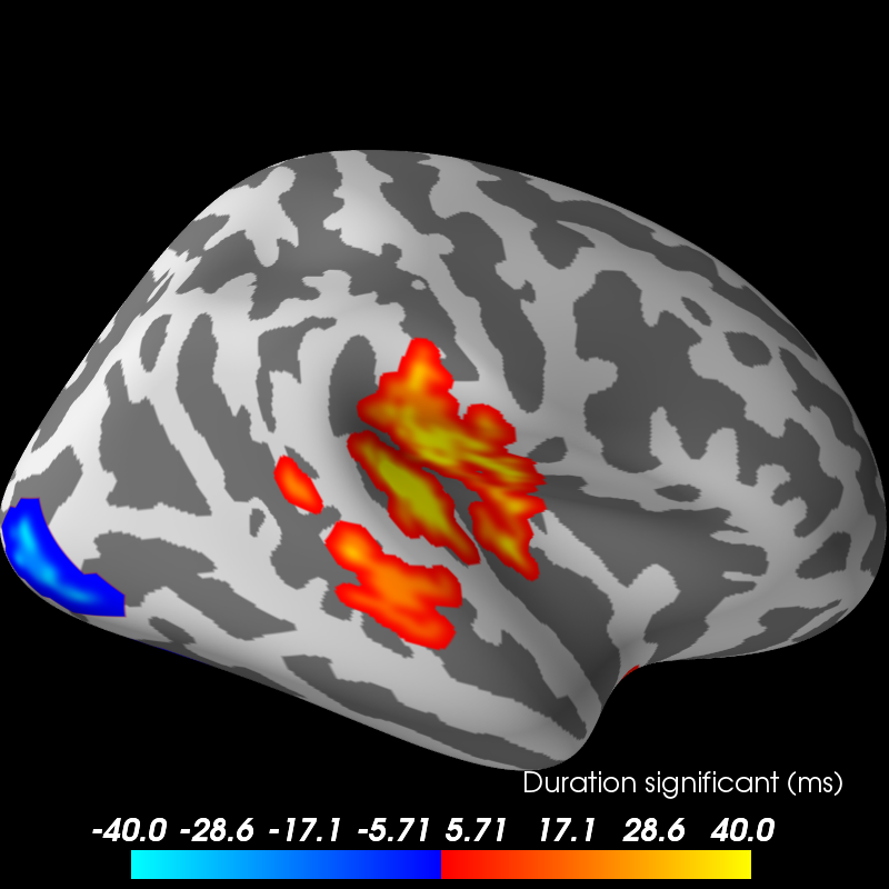
# Let's actually plot the first "time point" in the SourceEstimate, which
# shows all the clusters, weighted by duration
subjects_dir = op.join(data_path, 'subjects')
# blue blobs are for condition A < condition B, red for A > B
brain = stc_all_cluster_vis.plot(hemi='both', views='lateral',
subjects_dir=subjects_dir,
time_label='Duration significant (ms)')
brain.save_image('clusters.png')
Out:
Visualizing clusters.
Updating smoothing matrix, be patient..
Smoothing matrix creation, step 1
Smoothing matrix creation, step 2
Smoothing matrix creation, step 3
Smoothing matrix creation, step 4
Smoothing matrix creation, step 5
Smoothing matrix creation, step 6
Smoothing matrix creation, step 7
Smoothing matrix creation, step 8
Smoothing matrix creation, step 9
Smoothing matrix creation, step 10
colormap: fmin=-4.00e+01 fmid=0.00e+00 fmax=4.00e+01 transparent=0
Total running time of the script: ( 0 minutes 39.832 seconds)