Tests if the source space data are significantly different between 2 groups of subjects (simulated here using one subject’s data). The multiple comparisons problem is addressed with a cluster-level permutation test across space and time.
# Authors: Alexandre Gramfort <alexandre.gramfort@telecom-paristech.fr>
#          Eric Larson <larson.eric.d@gmail.com>
# License: BSD (3-clause)

import os.path as op

import numpy as np
from scipy import stats as stats

import mne
from mne import spatial_tris_connectivity, grade_to_tris
from mne.stats import spatio_temporal_cluster_test, summarize_clusters_stc
from mne.datasets import sample

print(__doc__)
data_path = sample.data_path()
stc_fname = data_path + '/MEG/sample/sample_audvis-meg-lh.stc'
subjects_dir = data_path + '/subjects'

# Load stc to in common cortical space (fsaverage)
stc = mne.read_source_estimate(stc_fname)
stc.resample(50, npad='auto')

stc = mne.morph_data('sample', 'fsaverage', stc, grade=5, smooth=20,
                     subjects_dir=subjects_dir)
n_vertices_fsave, n_times = stc.data.shape
tstep = stc.tstep

n_subjects1, n_subjects2 = 7, 9
print('Simulating data for %d and %d subjects.' % (n_subjects1, n_subjects2))

#    Let's make sure our results replicate, so set the seed.
np.random.seed(0)
X1 = np.random.randn(n_vertices_fsave, n_times, n_subjects1) * 10
X2 = np.random.randn(n_vertices_fsave, n_times, n_subjects2) * 10
X1[:, :, :] += stc.data[:, :, np.newaxis]
# make the activity bigger for the second set of subjects
X2[:, :, :] += 3 * stc.data[:, :, np.newaxis]

#    We want to compare the overall activity levels for each subject
X1 = np.abs(X1)  # only magnitude
X2 = np.abs(X2)  # only magnitude
Out:
Morphing data...
    Left-hemisphere map read.
    Right-hemisphere map read.
    20 smooth iterations done.
    20 smooth iterations done.
[done]
Simulating data for 7 and 9 subjects.
To use an algorithm optimized for spatio-temporal clustering, we just pass the spatial connectivity matrix (instead of spatio-temporal)
print('Computing connectivity.')
connectivity = spatial_tris_connectivity(grade_to_tris(5))

#    Note that X needs to be a list of multi-dimensional array of shape
#    samples (subjects_k) x time x space, so we permute dimensions
X1 = np.transpose(X1, [2, 1, 0])
X2 = np.transpose(X2, [2, 1, 0])
X = [X1, X2]

#    Now let's actually do the clustering. This can take a long time...
#    Here we set the threshold quite high to reduce computation.
p_threshold = 0.0001
f_threshold = stats.distributions.f.ppf(1. - p_threshold / 2.,
                                        n_subjects1 - 1, n_subjects2 - 1)
print('Clustering.')
T_obs, clusters, cluster_p_values, H0 = clu =\
    spatio_temporal_cluster_test(X, connectivity=connectivity, n_jobs=1,
                                 threshold=f_threshold)
#    Now select the clusters that are sig. at p < 0.05 (note that this value
#    is multiple-comparisons corrected).
good_cluster_inds = np.where(cluster_p_values < 0.05)[0]
Out:
Computing connectivity.
-- number of connected vertices : 20484
Clustering.
stat_fun(H1): min=0.000000 max=279.936851
Running initial clustering
Found 224 clusters
Permuting ...

[                                        ] 0.09766 |
[.                                       ] 3.12500 /
[..                                      ] 6.25000 -
[...                                     ] 9.37500 \
[.....                                   ] 12.50000 |
[......                                  ] 15.62500 /
[.......                                 ] 18.75000 -
[........                                ] 21.87500 \
[..........                              ] 25.00000 |
[...........                             ] 28.12500 /
[............                            ] 31.25000 -
[.............                           ] 34.37500 \
[...............                         ] 37.50000 |
[................                        ] 40.62500 /
[.................                       ] 43.75000 -
[..................                      ] 46.87500 \
[....................                    ] 50.00000 |
[.....................                   ] 53.12500 /
[......................                  ] 56.25000 -
[.......................                 ] 59.37500 \
[.........................               ] 62.50000 |
[..........................              ] 65.62500 /
[...........................             ] 68.75000 -
[............................            ] 71.87500 \
[..............................          ] 75.00000 |
[...............................         ] 78.12500 /
[................................        ] 81.25000 -
[.................................       ] 84.37500 \
[...................................     ] 87.50000 |
[....................................    ] 90.62500 /
[.....................................   ] 93.75000 -
[......................................  ] 96.87500 \
[........................................] 100.00000 |    Computing cluster p-values
Done.
print('Visualizing clusters.')
# Now let's build a convenient representation of each cluster, where each
# cluster becomes a "time point" in the SourceEstimate
fsave_vertices = [np.arange(10242), np.arange(10242)]
stc_all_cluster_vis = summarize_clusters_stc(clu, tstep=tstep,
vertices=fsave_vertices,
subject='fsaverage')
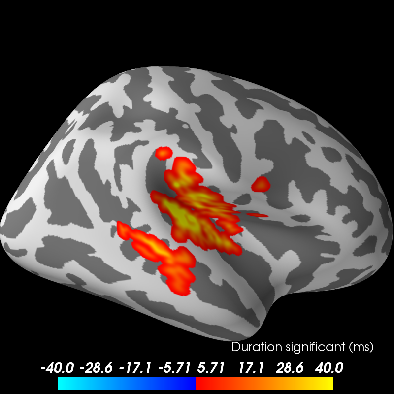
# Let's actually plot the first "time point" in the SourceEstimate, which
# shows all the clusters, weighted by duration
subjects_dir = op.join(data_path, 'subjects')
# blue blobs are for condition A != condition B
brain = stc_all_cluster_vis.plot('fsaverage', hemi='both', colormap='mne',
views='lateral', subjects_dir=subjects_dir,
time_label='Duration significant (ms)')
brain.save_image('clusters.png')
Out:
Visualizing clusters.
Updating smoothing matrix, be patient..
Smoothing matrix creation, step 1
Smoothing matrix creation, step 2
Smoothing matrix creation, step 3
Smoothing matrix creation, step 4
Smoothing matrix creation, step 5
Smoothing matrix creation, step 6
Smoothing matrix creation, step 7
Smoothing matrix creation, step 8
Smoothing matrix creation, step 9
Smoothing matrix creation, step 10
colormap: fmin=-4.00e+01 fmid=0.00e+00 fmax=4.00e+01 transparent=0
Total running time of the script: ( 3 minutes 30.205 seconds)