Tests for differential evoked responses in at least one condition using a permutation clustering test. The FieldTrip neighbor templates will be used to determine the adjacency between sensors. This serves as a spatial prior to the clustering. Significant spatiotemporal clusters will then be visualized using custom matplotlib code.
# Authors: Denis Engemann <denis.engemann@gmail.com>
#
# License: BSD (3-clause)

import numpy as np
import matplotlib.pyplot as plt
from mpl_toolkits.axes_grid1 import make_axes_locatable
from mne.viz import plot_topomap

import mne
from mne.stats import spatio_temporal_cluster_test
from mne.datasets import sample
from mne.channels import read_ch_connectivity

print(__doc__)
data_path = sample.data_path()
raw_fname = data_path + '/MEG/sample/sample_audvis_filt-0-40_raw.fif'
event_fname = data_path + '/MEG/sample/sample_audvis_filt-0-40_raw-eve.fif'
event_id = {'Aud_L': 1, 'Aud_R': 2, 'Vis_L': 3, 'Vis_R': 4}
tmin = -0.2
tmax = 0.5

# Setup for reading the raw data
raw = mne.io.read_raw_fif(raw_fname, preload=True)
raw.filter(1, 30, l_trans_bandwidth='auto', h_trans_bandwidth='auto',
           filter_length='auto', phase='zero')
events = mne.read_events(event_fname)
Out:
Opening raw data file /home/ubuntu/mne_data/MNE-sample-data/MEG/sample/sample_audvis_filt-0-40_raw.fif...
    Read a total of 4 projection items:
        PCA-v1 (1 x 10²)  idle
        PCA-v2 (1 x 10²)  idle
        PCA-v3 (1 x 10²)  idle
        Average EEG reference (1 x 60)  idle
    Range : 6450 ... 48149 =     42.956 ...   320.665 secs
Ready.
Current compensation grade : 0
Reading 0 ... 41699  =      0.000 ...   277.709 secs...
Setting up band-pass filter from 1 - 30 Hz
l_trans_bandwidth chosen to be 1.0 Hz
h_trans_bandwidth chosen to be 7.5 Hz
Filter length of 991 samples (6.600 sec) selected
picks = mne.pick_types(raw.info, meg='mag', eog=True)

reject = dict(mag=4e-12, eog=150e-6)
epochs = mne.Epochs(raw, events, event_id, tmin, tmax, picks=picks,
                    baseline=None, reject=reject, preload=True)

epochs.drop_channels(['EOG 061'])
epochs.equalize_event_counts(event_id)

condition_names = 'Aud_L', 'Aud_R', 'Vis_L', 'Vis_R'
X = [epochs[k].get_data() for k in condition_names]  # as 3D matrix
X = [np.transpose(x, (0, 2, 1)) for x in X]  # transpose for clustering
Out:
288 matching events found
Created an SSP operator (subspace dimension = 3)
4 projection items activated
Loading data for 288 events and 106 original time points ...
    Rejecting  epoch based on EOG : [u'EOG 061']
    Rejecting  epoch based on EOG : [u'EOG 061']
    Rejecting  epoch based on EOG : [u'EOG 061']
    Rejecting  epoch based on EOG : [u'EOG 061']
    Rejecting  epoch based on EOG : [u'EOG 061']
    Rejecting  epoch based on EOG : [u'EOG 061']
    Rejecting  epoch based on EOG : [u'EOG 061']
    Rejecting  epoch based on EOG : [u'EOG 061']
    Rejecting  epoch based on EOG : [u'EOG 061']
    Rejecting  epoch based on EOG : [u'EOG 061']
    Rejecting  epoch based on EOG : [u'EOG 061']
    Rejecting  epoch based on EOG : [u'EOG 061']
    Rejecting  epoch based on EOG : [u'EOG 061']
    Rejecting  epoch based on EOG : [u'EOG 061']
    Rejecting  epoch based on EOG : [u'EOG 061']
    Rejecting  epoch based on MAG : [u'MEG 1711']
    Rejecting  epoch based on EOG : [u'EOG 061']
    Rejecting  epoch based on EOG : [u'EOG 061']
    Rejecting  epoch based on EOG : [u'EOG 061']
    Rejecting  epoch based on EOG : [u'EOG 061']
    Rejecting  epoch based on EOG : [u'EOG 061']
    Rejecting  epoch based on MAG : [u'MEG 1711']
    Rejecting  epoch based on EOG : [u'EOG 061']
    Rejecting  epoch based on EOG : [u'EOG 061']
    Rejecting  epoch based on EOG : [u'EOG 061']
    Rejecting  epoch based on EOG : [u'EOG 061']
    Rejecting  epoch based on EOG : [u'EOG 061']
    Rejecting  epoch based on EOG : [u'EOG 061']
    Rejecting  epoch based on EOG : [u'EOG 061']
    Rejecting  epoch based on EOG : [u'EOG 061']
    Rejecting  epoch based on EOG : [u'EOG 061']
    Rejecting  epoch based on EOG : [u'EOG 061']
    Rejecting  epoch based on EOG : [u'EOG 061']
    Rejecting  epoch based on EOG : [u'EOG 061']
    Rejecting  epoch based on EOG : [u'EOG 061']
    Rejecting  epoch based on EOG : [u'EOG 061']
    Rejecting  epoch based on EOG : [u'EOG 061']
    Rejecting  epoch based on EOG : [u'EOG 061']
    Rejecting  epoch based on EOG : [u'EOG 061']
    Rejecting  epoch based on EOG : [u'EOG 061']
    Rejecting  epoch based on EOG : [u'EOG 061']
    Rejecting  epoch based on EOG : [u'EOG 061']
    Rejecting  epoch based on EOG : [u'EOG 061']
    Rejecting  epoch based on EOG : [u'EOG 061']
    Rejecting  epoch based on EOG : [u'EOG 061']
    Rejecting  epoch based on EOG : [u'EOG 061']
    Rejecting  epoch based on EOG : [u'EOG 061']
    Rejecting  epoch based on EOG : [u'EOG 061']
    Rejecting  epoch based on EOG : [u'EOG 061']
49 bad epochs dropped
Dropped 19 epochs
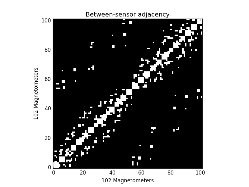
connectivity, ch_names = read_ch_connectivity('neuromag306mag')

print(type(connectivity))  # it's a sparse matrix!

plt.imshow(connectivity.toarray(), cmap='gray', origin='lower',
           interpolation='nearest')
plt.xlabel('{} Magnetometers'.format(len(ch_names)))
plt.ylabel('{} Magnetometers'.format(len(ch_names)))
plt.title('Between-sensor adjacency')
Out:
<class 'scipy.sparse.csr.csr_matrix'>
How does it work? We use clustering to bind together features which are similar. Our features are the magnetic fields measured over our sensor array at different times. This reduces the multiple comparison problem. To compute the actual test-statistic, we first sum all F-values in all clusters. We end up with one statistic for each cluster. Then we generate a distribution from the data by shuffling our conditions between our samples and recomputing our clusters and the test statistics. We test for the significance of a given cluster by computing the probability of observing a cluster of that size. For more background read: Maris/Oostenveld (2007), “Nonparametric statistical testing of EEG- and MEG-data” Journal of Neuroscience Methods, Vol. 164, No. 1., pp. 177-190. doi:10.1016/j.jneumeth.2007.03.024
# set cluster threshold
threshold = 50.0  # very high, but the test is quite sensitive on this data
# set family-wise p-value
p_accept = 0.001

cluster_stats = spatio_temporal_cluster_test(X, n_permutations=1000,
                                             threshold=threshold, tail=1,
                                             n_jobs=1,
                                             connectivity=connectivity)

T_obs, clusters, p_values, _ = cluster_stats
good_cluster_inds = np.where(p_values < p_accept)[0]
Out:
stat_fun(H1): min=0.003978 max=192.417886
Running initial clustering
Found 7 clusters
Permuting ...

[                                        ] 0.10000 |
[.                                       ] 3.20000 /
[..                                      ] 6.40000 -
[...                                     ] 9.60000 \
[.....                                   ] 12.80000 |
[......                                  ] 16.00000 /
[.......                                 ] 19.20000 -
[........                                ] 22.40000 \
[..........                              ] 25.60000 |
[...........                             ] 28.80000 /
[............                            ] 32.00000 -
[..............                          ] 35.20000 \
[...............                         ] 38.40000 |
[................                        ] 41.60000 /
[.................                       ] 44.80000 -
[...................                     ] 48.00000 \
[....................                    ] 51.20000 |
[.....................                   ] 54.40000 /
[.......................                 ] 57.60000 -
[........................                ] 60.80000 \
[.........................               ] 64.00000 |
[..........................              ] 67.20000 /
[............................            ] 70.40000 -
[.............................           ] 73.60000 \
[..............................          ] 76.80000 |
[................................        ] 80.00000 /
[.................................       ] 83.20000 -
[..................................      ] 86.40000 \
[...................................     ] 89.60000 |
[.....................................   ] 92.80000 /
[......................................  ] 96.00000 -
[....................................... ] 99.20000 \    Computing cluster p-values
Done.
Note. The same functions work with source estimate. The only differences are the origin of the data, the size, and the connectivity definition. It can be used for single trials or for groups of subjects.
# configure variables for visualization
times = epochs.times * 1e3
colors = 'r', 'r', 'steelblue', 'steelblue'
linestyles = '-', '--', '-', '--'
# grand average as numpy arrray
grand_ave = np.array(X).mean(axis=1)
# get sensor positions via layout
pos = mne.find_layout(epochs.info).pos
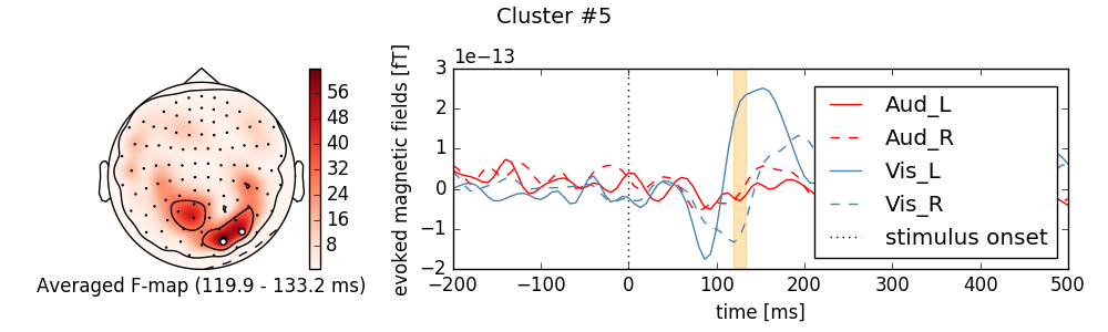
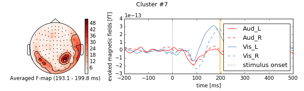
# loop over significant clusters
for i_clu, clu_idx in enumerate(good_cluster_inds):
# unpack cluster information, get unique indices
time_inds, space_inds = np.squeeze(clusters[clu_idx])
ch_inds = np.unique(space_inds)
time_inds = np.unique(time_inds)
# get topography for F stat
f_map = T_obs[time_inds, ...].mean(axis=0)
# get signals at significant sensors
signals = grand_ave[..., ch_inds].mean(axis=-1)
sig_times = times[time_inds]
# create spatial mask
mask = np.zeros((f_map.shape[0], 1), dtype=bool)
mask[ch_inds, :] = True
# initialize figure
fig, ax_topo = plt.subplots(1, 1, figsize=(10, 3))
title = 'Cluster #{0}'.format(i_clu + 1)
fig.suptitle(title, fontsize=14)
# plot average test statistic and mark significant sensors
image, _ = plot_topomap(f_map, pos, mask=mask, axes=ax_topo,
cmap='Reds', vmin=np.min, vmax=np.max)
# advanced matplotlib for showing image with figure and colorbar
# in one plot
divider = make_axes_locatable(ax_topo)
# add axes for colorbar
ax_colorbar = divider.append_axes('right', size='5%', pad=0.05)
plt.colorbar(image, cax=ax_colorbar)
ax_topo.set_xlabel('Averaged F-map ({:0.1f} - {:0.1f} ms)'.format(
*sig_times[[0, -1]]
))
# add new axis for time courses and plot time courses
ax_signals = divider.append_axes('right', size='300%', pad=1.2)
for signal, name, col, ls in zip(signals, condition_names, colors,
linestyles):
ax_signals.plot(times, signal, color=col, linestyle=ls, label=name)
# add information
ax_signals.axvline(0, color='k', linestyle=':', label='stimulus onset')
ax_signals.set_xlim([times[0], times[-1]])
ax_signals.set_xlabel('time [ms]')
ax_signals.set_ylabel('evoked magnetic fields [fT]')
# plot significant time range
ymin, ymax = ax_signals.get_ylim()
ax_signals.fill_betweenx((ymin, ymax), sig_times[0], sig_times[-1],
color='orange', alpha=0.3)
ax_signals.legend(loc='lower right')
ax_signals.set_ylim(ymin, ymax)
# clean up viz
mne.viz.tight_layout(fig=fig)
fig.subplots_adjust(bottom=.05)
plt.show()


scipy.stats.distributions.fTotal running time of the script: ( 0 minutes 25.847 seconds)