Many M/EEG signals including biological artifacts reflect non-Gaussian
processes. Therefore PCA-based artifact rejection will likely perform worse at
separating the signal from noise sources.
MNE-Python supports identifying artifacts and latent components using temporal ICA.
MNE-Python implements the mne.preprocessing.ICA class that facilitates applying ICA
to MEG and EEG data. It supports FastICA, the infomax, and the extended informax algorithm.
It allows whitening the data using a fast randomized PCA algorithmd. Furthermore,
multiple sensor types are supported by pre-whitening / rescaling. Bad data segments can be excluded
from the model fitting by reject parameter in mne.preprocessing.ICA.fit.
mne.preprocessing.ICA implements methods formne.preprocessing.ICA.plot_components() for mapping the spatial sensitvity of a comopnentmne.preprocessing.ICA.plot_sources() for component related time seriesmne.preprocessing.ICA.plot_scores() for scores on which component detection is based uponmne.preprocessing.ICA.plot_overlay() for showing differences between raw and processed datamne.preprocessing.ICA.save() for writing the ICA solution into a fif file.mne.preprocessing.ICA.get_sources() for putting component related time series in MNE data structures.ICA finds directions in the feature space corresponding to projections with high non-Gaussianity.
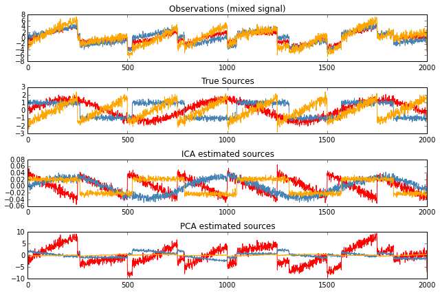
Example: Imagine 3 instruments playing simultaneously and 3 microphones recording mixed signals. ICA can be used to recover the sources ie. what is played by each instrument.
ICA employs a very simple model: $X = AS$ where $X$ is our observations, $A$ is the mixing matrix and $S$ is the vector of independent (latent) sources.
The challenge is to recover A and S from X.
import numpy as np
import matplotlib.pyplot as plt
from scipy import signal

from sklearn.decomposition import FastICA, PCA

np.random.seed(0)  # set seed for reproducible results
n_samples = 2000
time = np.linspace(0, 8, n_samples)

s1 = np.sin(2 * time)  # Signal 1 : sinusoidal signal
s2 = np.sign(np.sin(3 * time))  # Signal 2 : square signal
s3 = signal.sawtooth(2 * np.pi * time)  # Signal 3: sawtooth signal

S = np.c_[s1, s2, s3]
S += 0.2 * np.random.normal(size=S.shape)  # Add noise

S /= S.std(axis=0)  # Standardize data
# Mix data
A = np.array([[1, 1, 1], [0.5, 2, 1.0], [1.5, 1.0, 2.0]])  # Mixing matrix
X = np.dot(S, A.T)  # Generate observations
# compute ICA
ica = FastICA(n_components=3)
S_ = ica.fit_transform(X)  # Get the estimated sources
A_ = ica.mixing_  # Get estimated mixing matrix

# compute PCA
pca = PCA(n_components=3)
H = pca.fit_transform(X)  # estimate PCA sources

plt.figure(figsize=(9, 6))

models = [X, S, S_, H]
names = ['Observations (mixed signal)',
         'True Sources',
         'ICA estimated sources',
         'PCA estimated sources']
colors = ['red', 'steelblue', 'orange']

for ii, (model, name) in enumerate(zip(models, names), 1):
    plt.subplot(4, 1, ii)
    plt.title(name)
    for sig, color in zip(model.T, colors):
        plt.plot(sig, color=color)

plt.tight_layout()
plt.show()

\(\rightarrow\) PCA fails at recovering our “instruments” since the related signals reflect non-Gaussian processes.