Projections¶

What is SSP?¶

Without loss of generality we can always decompose any \(n\)-channel measurement \(b(t)\) into its signal and noise components as

Further, if we know that \(b_n(t)\) is well characterized by a few field patterns \(b_1 \dotso b_m\), we can express the disturbance as

where the columns of \(U\) constitute an orthonormal basis for \(b_1 \dotso b_m\), \(c_n(t)\) is an \(m\)-component column vector, and the error term \(e(t)\) is small and does not exhibit any consistent spatial distributions over time, i.e., \(C_e = E \{e e^T\} = I\). Subsequently, we will call the column space of \(U\) the noise subspace. The basic idea of SSP is that we can actually find a small basis set \(b_1 \dotso b_m\) such that the conditions described above are satisfied. We can now construct the orthogonal complement operator

and apply it to \(b(t)\) in Equation (1) yielding

since \(P_{\perp}b_n(t) = P_{\perp}(Uc_n(t) + e(t)) \approx 0\) and \(P_{\perp}b_{s}(t) \approx b_{s}(t)\). The projection operator \(P_{\perp}\) is called the signal-space projection operator.

Why SSP?¶

It provides considerable rejection of noise, suppressing external disturbances by a factor of 10 or more. The effectiveness of SSP depends on two factors:

• The basis set \(b_1 \dotso b_m\) should be able to characterize the disturbance field patterns completely and
• The angles between the noise subspace space spanned by \(b_1 \dotso b_m\) and the signal vectors \(b_s(t)\) should be as close to \(\pi / 2\) as possible.

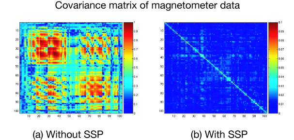
If the first requirement is not satisfied, some noise will leak through because \(P_{\perp}b_n(t) \neq 0\). If the any of the brain signal vectors \(b_s(t)\) is close to the noise subspace not only the noise but also the signal will be attenuated by the application of \(P_{\perp}\) and, consequently, there might by little gain in signal-to-noise ratio. An example of the effect of SSP demonstrates the effect of SSP on the Vectorview magnetometer data. After the elimination of a three-dimensional noise subspace, the absolute value of the noise is dampened approximately by a factor of 10 and the covariance matrix becomes diagonally dominant.

Since the signal-space projection modifies the signal vectors originating in the brain, it is necessary to apply the projection to the forward solution in the course of inverse computations. This is accomplished by mne_inverse_operator as described in Inverse-operator decomposition. For more information on SSP, please consult the references listed in Signal-space projections.

An example of the effect of SSP

The covariance matrix \(C_n\) of noise data on the 102 Vectorview magnetometers was computed (a) before and (b) after the application of SSP with three-dimensional noise subspace. The plotted quantity is \(\sqrt {|(C_n)_{jk}|}\). Note that the vertical scale in (b) is ten times smaller than in (a).

Estimation of the noise subspace¶

As described above, application of SSP requires the estimation of the signal vectors \(b_1 \dotso b_m\) constituting the noise subspace. The most common approach, also implemented in mne_browse_raw is to compute a covariance matrix of empty room data, compute its eigenvalue decomposition, and employ the eigenvectors corresponding to the highest eigenvalues as basis for the noise subspace. It is also customary to use a separate set of vectors for magnetometers and gradiometers in the Vectorview system.

Average reference¶

The EEG average reference is the mean signal over all the sensors. It is typical in EEG analysis to subtract the average reference from all the sensor signals \(b^{1}(t), ..., b^{n}(t)\). That is:

where the noise term \(b_{n}^{j}(t)\) is given by

Thus, the projector vector \(P_{\perp}\) will be given by \(P_{\perp}=\frac{1}{n}[1, 1, ..., 1]\)

The proj attribute¶

It is available in all the basic data containers: Raw, Epochs and Evoked. It is True if at least one projector is present and all of them are active.

Computing projectors¶

In MNE-Python SSP vectors can be computed using general purpose functions mne.compute_proj_epochs(), mne.compute_proj_evoked(), and mne.compute_proj_raw(). The general assumption these functions make is that the data passed contains raw, epochs or averages of the artifact. Typically this involves continues raw data of empty room recordings or averaged ECG or EOG artifacts.

A second set of highlevel convenience functions is provided to compute projection vector for typical usecases. This includes mne.preprocessing.compute_proj_ecg() and mne.preprocessing.compute_proj_eog() for computing the ECG and EOG related artifact components, respectively. For computing the EEG reference signal, the function mne.set_eeg_reference() can be used.

Adding/removing projectors¶

To explicitly add a proj, use add_proj. For example:

>>> projs = mne.read_proj('proj_a.fif')
>>> evoked.add_proj(projs)

If projectors are already present in the raw fif file, it will be added to the info dictionary automatically. To remove existing projectors, you can do:

>>> evoked.add_proj([], remove_existing=True)

Applying projectors¶

Projectors can be applied at any stage of the pipeline. When the raw data is read in, the projectors are not applied by default but this flag can be turned on. However, at the epochs stage, the projectors are applied by default.

To apply explicitly projs at any stage of the pipeline, use apply_proj. For example:

>>> evoked.apply_proj()

The projectors might not be applied if data are not preloaded. In this case, it’s the _projector attribute that indicates if a projector will be applied when the data is loaded in memory. If the data is already in memory, then the projectors applied to it are the ones marked as active. As soon as you’ve applied the projectors, it will stay active in the remaining pipeline.

Delayed projectors¶

The suggested pipeline is proj=True in epochs (it’s computationally cheaper than for raw). When you use delayed SSP in Epochs, projectors are applied when you call mne.Epochs.get_data() method. They are not applied to the evoked data unless you call apply_proj(). The reason is that you want to reject epochs with projectors although it’s not stored in the projector mode.