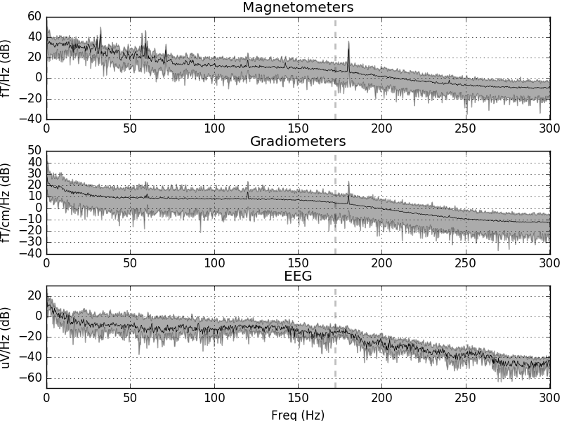
This script shows how to compute the power spectral density (PSD) of measurements on a raw dataset. It also show the effect of applying SSP to the data to reduce ECG and EOG artifacts.
# Authors: Alexandre Gramfort <alexandre.gramfort@telecom-paristech.fr>
#          Martin Luessi <mluessi@nmr.mgh.harvard.edu>
#          Eric Larson <larson.eric.d@gmail.com>
# License: BSD (3-clause)

import numpy as np
import matplotlib.pyplot as plt

import mne
from mne import io, read_proj, read_selection
from mne.datasets import sample
from mne.time_frequency import psd_multitaper

print(__doc__)
Set parameters
data_path = sample.data_path()
raw_fname = data_path + '/MEG/sample/sample_audvis_raw.fif'
proj_fname = data_path + '/MEG/sample/sample_audvis_eog-proj.fif'
tmin, tmax = 0, 60 # use the first 60s of data
# Setup for reading the raw data (to save memory, crop before loading)
raw = io.read_raw_fif(raw_fname).crop(tmin, tmax).load_data()
raw.info['bads'] += ['MEG 2443', 'EEG 053'] # bads + 2 more
# Add SSP projection vectors to reduce EOG and ECG artifacts
projs = read_proj(proj_fname)
raw.add_proj(projs, remove_existing=True)
fmin, fmax = 2, 300 # look at frequencies between 2 and 300Hz
n_fft = 2048 # the FFT size (n_fft). Ideally a power of 2
# Let's first check out all channel types
raw.plot_psd(area_mode='range', tmax=10.0, show=False)
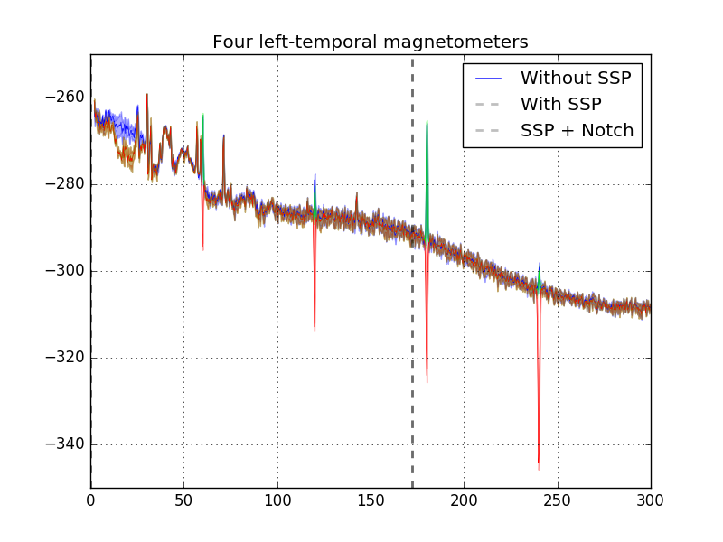
# Now let's focus on a smaller subset:
# Pick MEG magnetometers in the Left-temporal region
selection = read_selection('Left-temporal')
picks = mne.pick_types(raw.info, meg='mag', eeg=False, eog=False,
stim=False, exclude='bads', selection=selection)
# Let's just look at the first few channels for demonstration purposes
picks = picks[:4]
plt.figure()
ax = plt.axes()
raw.plot_psd(tmin=tmin, tmax=tmax, fmin=fmin, fmax=fmax, n_fft=n_fft,
n_jobs=1, proj=False, ax=ax, color=(0, 0, 1), picks=picks,
show=False)
# And now do the same with SSP applied
raw.plot_psd(tmin=tmin, tmax=tmax, fmin=fmin, fmax=fmax, n_fft=n_fft,
n_jobs=1, proj=True, ax=ax, color=(0, 1, 0), picks=picks,
show=False)
# And now do the same with SSP + notch filtering
# Pick all channels for notch since the SSP projection mixes channels together
raw.notch_filter(np.arange(60, 241, 60), n_jobs=1)
raw.plot_psd(tmin=tmin, tmax=tmax, fmin=fmin, fmax=fmax, n_fft=n_fft,
n_jobs=1, proj=True, ax=ax, color=(1, 0, 0), picks=picks,
show=False)
ax.set_title('Four left-temporal magnetometers')
plt.legend(['Without SSP', 'With SSP', 'SSP + Notch'])
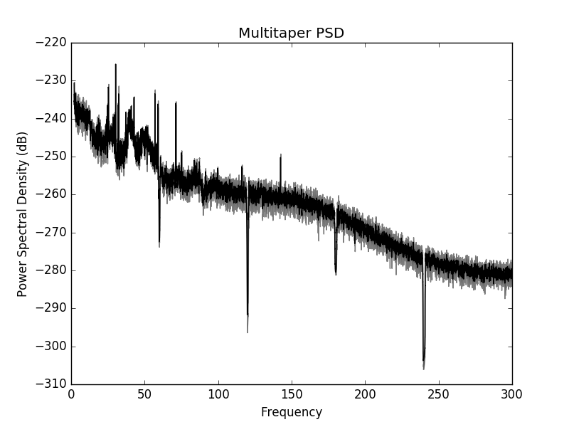
# Alternatively, you may also create PSDs from Raw objects with ``psd_*``
f, ax = plt.subplots()
psds, freqs = psd_multitaper(raw, low_bias=True, tmin=tmin, tmax=tmax,
fmin=fmin, fmax=fmax, proj=True, picks=picks,
n_jobs=1)
psds = 10 * np.log10(psds)
psds_mean = psds.mean(0)
psds_std = psds.std(0)
ax.plot(freqs, psds_mean, color='k')
ax.fill_between(freqs, psds_mean - psds_std, psds_mean + psds_std,
color='k', alpha=.5)
ax.set(title='Multitaper PSD', xlabel='Frequency',
ylabel='Power Spectral Density (dB)')
plt.show()
Out:
Opening raw data file /home/ubuntu/mne_data/MNE-sample-data/MEG/sample/sample_audvis_raw.fif...
    Read a total of 3 projection items:
        PCA-v1 (1 x 10²)  idle
        PCA-v2 (1 x 10²)  idle
        PCA-v3 (1 x 10²)  idle
    Range : 25800 ... 192599 =     42.956 ...   320.670 secs
Ready.
Current compensation grade : 0
Reading 0 ... 36037  =      0.000 ...    60.000 secs...
    Read a total of 6 projection items:
        EOG-planar-998--0.200-0.200-PCA-01 (1 x 203)  idle
        EOG-planar-998--0.200-0.200-PCA-02 (1 x 203)  idle
        EOG-axial-998--0.200-0.200-PCA-01 (1 x 10²)  idle
        EOG-axial-998--0.200-0.200-PCA-02 (1 x 10²)  idle
        EOG-eeg-998--0.200-0.200-PCA-01 (1 x 59)  idle
        EOG-eeg-998--0.200-0.200-PCA-02 (1 x 59)  idle
6 projection items deactivated
Effective window size : 3.410 (s)
Effective window size : 3.410 (s)
Effective window size : 3.410 (s)
Effective window size : 3.410 (s)
Adding average EEG reference projection.
Created an SSP operator (subspace dimension = 7)
7 projection items activated
SSP projectors applied...
Effective window size : 3.410 (s)
Setting up band-stop filter
Filter length of 7928 samples (13.200 sec) selected
Adding average EEG reference projection.
Created an SSP operator (subspace dimension = 7)
7 projection items activated
SSP projectors applied...
Effective window size : 3.410 (s)
Adding average EEG reference projection.
Created an SSP operator (subspace dimension = 7)
7 projection items activated
SSP projectors applied...
Total running time of the script: ( 0 minutes 7.863 seconds)