Load evoked data and plot topomaps for selected time points.

Out:
Reading /home/ubuntu/mne_data/MNE-sample-data/MEG/sample/sample_audvis-ave.fif ...
    Read a total of 4 projection items:
        PCA-v1 (1 x 10²) active
        PCA-v2 (1 x 10²) active
        PCA-v3 (1 x 10²) active
        Average EEG reference (1 x 60) active
    Found the data of interest:
        t =    -199.80 ...     499.49 ms (Left Auditory)
        0 CTF compensation matrices available
        nave = 55 - aspect type = 100
Projections have already been applied. Setting proj attribute to True.
Applying baseline correction (mode: mean)
Initializing animation...
# Authors: Christian Brodbeck <christianbrodbeck@nyu.edu>
# Tal Linzen <linzen@nyu.edu>
# Denis A. Engeman <denis.engemann@gmail.com>
#
# License: BSD (3-clause)
import numpy as np
import matplotlib.pyplot as plt
from mne.datasets import sample
from mne import read_evokeds
print(__doc__)
path = sample.data_path()
fname = path + '/MEG/sample/sample_audvis-ave.fif'
# load evoked and subtract baseline
condition = 'Left Auditory'
evoked = read_evokeds(fname, condition=condition, baseline=(None, 0))
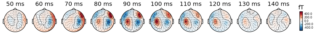
# set time instants in seconds (from 50 to 150ms in a step of 10ms)
times = np.arange(0.05, 0.15, 0.01)
# If times is set to None only 10 regularly spaced topographies will be shown
# plot magnetometer data as topomaps
evoked.plot_topomap(times, ch_type='mag')
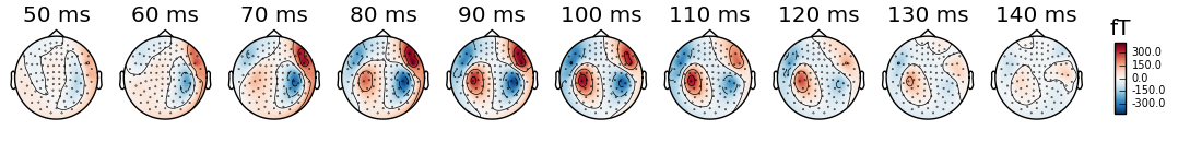
# compute a 50 ms bin to stabilize topographies
evoked.plot_topomap(times, ch_type='mag', average=0.05)
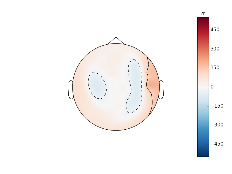
# plot gradiometer data (plots the RMS for each pair of gradiometers)
evoked.plot_topomap(times, ch_type='grad')
# plot magnetometer data as an animation
evoked.animate_topomap(ch_type='mag', times=times, frame_rate=10)
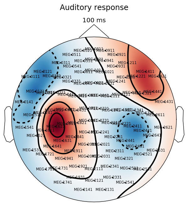
# plot magnetometer data as topomap at 1 time point : 100 ms
# and add channel labels and title
evoked.plot_topomap(0.1, ch_type='mag', show_names=True, colorbar=False,
size=6, res=128, title='Auditory response')
plt.subplots_adjust(left=0.01, right=0.99, bottom=0.01, top=0.88)
Total running time of the script: ( 0 minutes 15.634 seconds)