The objective is to show you how to explore the spectral content of your data (frequency and time-frequency). Here we’ll work on Epochs.
We will use the somatosensory dataset that contains so called event related synchronizations (ERS) / desynchronizations (ERD) in the beta band.
import numpy as np
import matplotlib.pyplot as plt

import mne
from mne.time_frequency import tfr_morlet, psd_multitaper
from mne.datasets import somato
Set parameters
data_path = somato.data_path()
raw_fname = data_path + '/MEG/somato/sef_raw_sss.fif'

# Setup for reading the raw data
raw = mne.io.read_raw_fif(raw_fname)
events = mne.find_events(raw, stim_channel='STI 014')

# picks MEG gradiometers
picks = mne.pick_types(raw.info, meg='grad', eeg=False, eog=True, stim=False)

# Construct Epochs
event_id, tmin, tmax = 1, -1., 3.
baseline = (None, 0)
epochs = mne.Epochs(raw, events, event_id, tmin, tmax, picks=picks,
                    baseline=baseline, reject=dict(grad=4000e-13, eog=350e-6),
                    preload=True)

epochs.resample(150., npad='auto')  # resample to reduce computation time
Out:
Opening raw data file /home/ubuntu/mne_data/MNE-somato-data/MEG/somato/sef_raw_sss.fif...
    Range : 237600 ... 506999 =    791.189 ...  1688.266 secs
Ready.
Current compensation grade : 0
111 events found
Events id: [1]
111 matching events found
0 projection items activated
Loading data for 111 events and 1202 original time points ...
    Rejecting  epoch based on EOG : [u'EOG 061']
    Rejecting  epoch based on EOG : [u'EOG 061']
    Rejecting  epoch based on EOG : [u'EOG 061']
3 bad epochs dropped
We start by exploring the frequence content of our epochs.
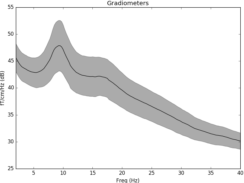
Let’s first check out all channel types by averaging across epochs.
epochs.plot_psd(fmin=2., fmax=40.)
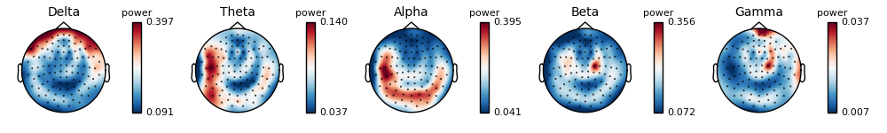
Now let’s take a look at the spatial distributions of the PSD.
epochs.plot_psd_topomap(ch_type='grad', normalize=True)
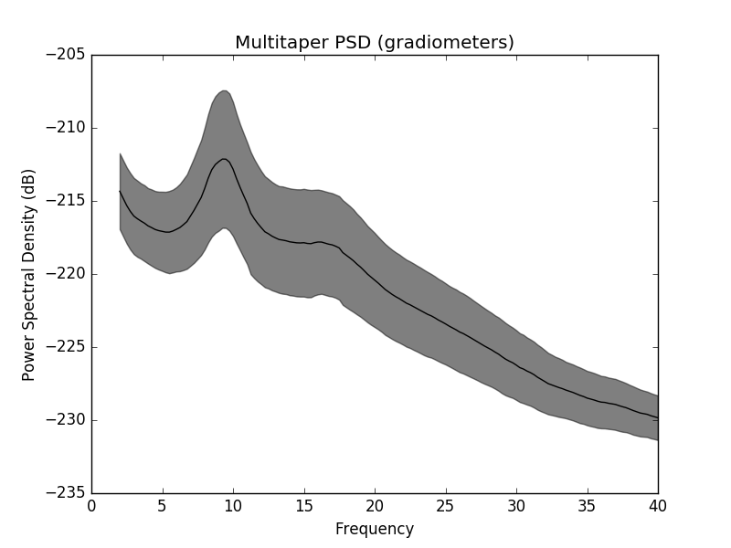
Alternatively, you can also create PSDs from Epochs objects with functions
that start with psd_ such as
mne.time_frequency.psd_multitaper() and
mne.time_frequency.psd_welch().
f, ax = plt.subplots()
psds, freqs = psd_multitaper(epochs, fmin=2, fmax=40, n_jobs=1)
psds = 10 * np.log10(psds)
psds_mean = psds.mean(0).mean(0)
psds_std = psds.mean(0).std(0)

ax.plot(freqs, psds_mean, color='k')
ax.fill_between(freqs, psds_mean - psds_std, psds_mean + psds_std,
                color='k', alpha=.5)
ax.set(title='Multitaper PSD (gradiometers)', xlabel='Frequency',
       ylabel='Power Spectral Density (dB)')
plt.show()
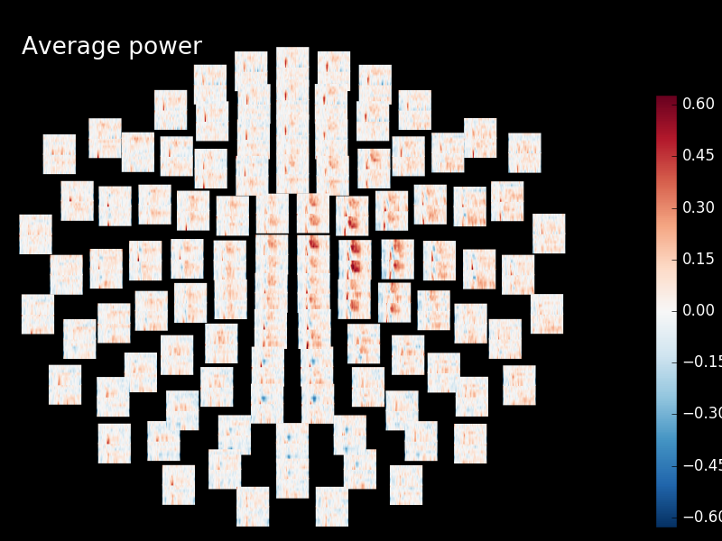
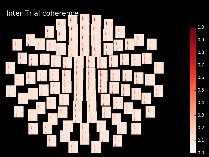
We now compute time-frequency representations (TFRs) from our Epochs. We’ll look at power and intertrial coherence (ITC).
To this we’ll use the function mne.time_frequency.tfr_morlet()
but you can also use mne.time_frequency.tfr_multitaper()
or mne.time_frequency.tfr_stockwell().
# define frequencies of interest (log-spaced)
freqs = np.logspace(*np.log10([6, 35]), num=8)
n_cycles = freqs / 2.  # different number of cycle per frequency
power, itc = tfr_morlet(epochs, freqs=freqs, n_cycles=n_cycles, use_fft=True,
                        return_itc=True, decim=3, n_jobs=1)
Note
The generated figures are interactive. In the topo you can click on an image to visualize the data for one censor. You can also select a portion in the time-frequency plane to obtain a topomap for a certain time-frequency region.
power.plot_topo(baseline=(-0.5, 0), mode='logratio', title='Average power')
power.plot([82], baseline=(-0.5, 0), mode='logratio')
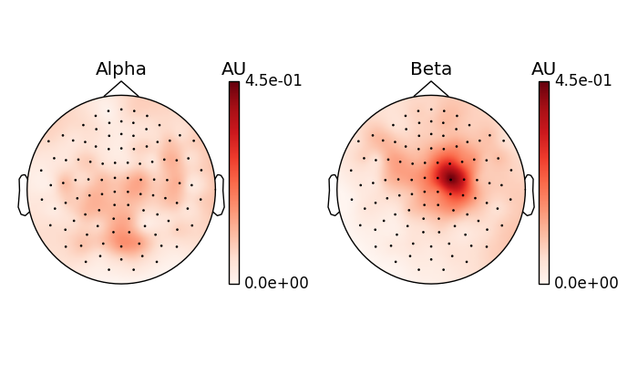
fig, axis = plt.subplots(1, 2, figsize=(7, 4))
power.plot_topomap(ch_type='grad', tmin=0.5, tmax=1.5, fmin=8, fmax=12,
baseline=(-0.5, 0), mode='logratio', axes=axis[0],
title='Alpha', vmax=0.45, show=False)
power.plot_topomap(ch_type='grad', tmin=0.5, tmax=1.5, fmin=13, fmax=25,
baseline=(-0.5, 0), mode='logratio', axes=axis[1],
title='Beta', vmax=0.45, show=False)
mne.viz.tight_layout()
plt.show()

Out:
Applying baseline correction (mode: logratio)
Applying baseline correction (mode: logratio)
Applying baseline correction (mode: logratio)
Applying baseline correction (mode: logratio)
itc.plot_topo(title='Inter-Trial coherence', vmin=0., vmax=1., cmap='Reds')
Out:
No baseline correction applied
Note
Baseline correction can be applied to power or done in plots To illustrate the baseline correction in plots the next line is commented power.apply_baseline(baseline=(-0.5, 0), mode=’logratio’)
- Visualize the intertrial coherence values as topomaps as done with power.
Total running time of the script: ( 0 minutes 34.606 seconds)