![]()
Contents
This Chapter covers the definitions of different coordinate systems employed in MNE software and FreeSurfer, the details of the computation of the forward solutions, and the associated low-level utilities.
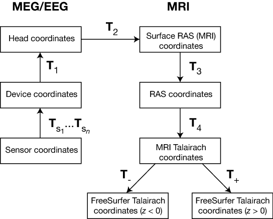
The coordinate systems used in MNE software (and FreeSurfer) and their relationships are depicted in MEG/EEG and MRI coordinate systems. Except for the Sensor coordinates, all of the coordinate systems are Cartesian and have the “RAS” (Right-Anterior-Superior) orientation, i.e., the \(x\) axis points to the right, the \(y\) axis to the front, and the \(z\) axis up.
MEG/EEG and MRI coordinate systems
The coordinate systems related to MEG/EEG data are:
Head coordinates
This is a coordinate system defined with help of the fiducial landmarks (nasion and the two auricular points). In fif files, EEG electrode locations are given in this coordinate system. In addition, the head digitization data acquired in the beginning of an MEG, MEG/EEG, or EEG acquisition are expressed in head coordinates. For details, see MEG/EEG and MRI coordinate systems.
Device coordinates
This is a coordinate system tied to the MEG device. The relationship of the Device and Head coordinates is determined during an MEG measurement by feeding current to three to five head-position indicator (HPI) coils and by determining their locations with respect to the MEG sensor array from the magnetic fields they generate.
Sensor coordinates
Each MEG sensor has a local coordinate system defining the orientation and location of the sensor. With help of this coordinate system, the numerical integration data needed for the computation of the magnetic field can be expressed conveniently as discussed in Coil geometry information. The channel information data in the fif files contain the information to specify the coordinate transformation between the coordinates of each sensor and the MEG device coordinates.
The coordinate systems related to MRI data are:
Surface RAS coordinates
The FreeSurfer surface data are expressed in this coordinate system. The origin of this coordinate system is at the center of the conformed FreeSurfer MRI volumes (usually 256 x 256 x 256 isotropic 1-mm3 voxels) and the axes are oriented along the axes of this volume. The BEM surface and the locations of the sources in the source space are usually expressed in this coordinate system in the fif files. In this manual, the Surface RAS coordinates are usually referred to as MRI coordinates unless there is need to specifically discuss the different MRI-related coordinate systems.
RAS coordinates
This coordinate system has axes identical to the Surface RAS coordinates but the location of the origin is different and defined by the original MRI data, i.e. , the origin is in a scanner-dependent location. There is hardly any need to refer to this coordinate system explicitly in the analysis with the MNE software. However, since the Talairach coordinates, discussed below, are defined with respect to RAS coordinates rather than the Surface RAS coordinates, the RAS coordinate system is implicitly involved in the transformation between Surface RAS coordinates and the two Talairach coordinate systems.
MNI Talairach coordinates
The definition of this coordinate system is discussed, e.g. , in http://imaging.mrc-cbu.cam.ac.uk/imaging/MniTalairach. This transformation is determined during the FreeSurfer reconstruction process.
FreeSurfer Talairach coordinates
The problem with the MNI Talairach coordinates is that the linear MNI Talairach transform does matched the brains completely to the Talairach brain. This is probably because the Talairach atlas brain is a rather odd shape, and as a result, it is difficult to match a standard brain to the atlas brain using an affine transform. As a result, the MNI brains are slightly larger (in particular higher, deeper and longer) than the Talairach brain. The differences are larger as you get further from the middle of the brain, towards the outside. The FreeSurfer Talairach coordinates mitigate this problem by additing a an additional transformation, defined separately for negatice and positive MNI Talairach \(z\) coordinates. These two transformations, denoted by \(T_-\) and \(T_+\) in MEG/EEG and MRI coordinate systems, are fixed as discussed in http://imaging.mrc-cbu.cam.ac.uk/imaging/MniTalairach (Approach 2).
The different coordinate systems are related by coordinate transformations depicted in MEG/EEG and MRI coordinate systems. The arrows and coordinate transformation symbols (\(T_x\)) indicate the transformations actually present in the FreeSurfer files. Generally,
where \(x_k\),:math:y_k,and \(z_k\) are the location coordinates in two coordinate systems, \(T_{12}\) is the coordinate transformation from coordinate system “1” to “2”, \(x_0\), \(y_0\),and \(z_0\) is the location of the origin of coordinate system “1” in coordinate system “2”, and \(R_{jk}\) are the elements of the rotation matrix relating the two coordinate systems. The coordinate transformations are present in different files produced by FreeSurfer and MNE as summarized in Coordinate transformations in FreeSurfer and MNE software packages.. The fixed transformations \(T_-\) and \(T_+\) are:
and
Note
This section does not discuss the transformation between the MRI voxel indices and the different MRI coordinates. However, it is important to note that in FreeSurfer, MNE, as well as in Neuromag software an integer voxel coordinate corresponds to the location of the center of a voxel. Detailed information on the FreeSurfer MRI systems can be found at https://surfer.nmr.mgh.harvard.edu/fswiki/CoordinateSystems.
| Transformation | FreeSurfer | MNE |
| \(T_1\) | Not present | Measurement data files
Forward solution files (*fwd.fif)
Inverse operator files (*inv.fif)
|
| \(T_{s_1}\dots T_{s_n}\) | Not present | Channel information in files containing \(T_1\). |
| \(T_2\) | Not present | MRI description files Separate
coordinate transformation files
saved from mne_analyze
Forward solution files
Inverse operator files
|
| \(T_3\) | mri/*mgz files | MRI description files saved with mne_make_cor_set if the input is in mgz or mgh format. |
| \(T_4\) | mri/transforms/talairach.xfm | MRI description files saved with mne_make_cor_set if the input is in mgz or mgh format. |
| \(T_-\) | Hardcoded in software | MRI description files saved with mne_make_cor_set if the input is in mgz or mgh format. |
| \(T_+\) | Hardcoded in software | MRI description files saved with mne_make_cor_set if the input is in mgz or mgh format. |
Note
The symbols \(T_x\) are defined in MEG/EEG and MRI coordinate systems. mne_make_cor_set /mne_setup_mri prior to release 2.6 did not include transformations \(T_3\), \(T_4\), \(T_-\), and \(T_+\) in the fif files produced.
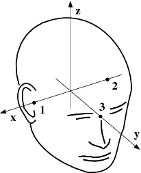
The head coordinate system
The MEG/EEG head coordinate system employed in the MNE software is a right-handed Cartesian coordinate system. The direction of \(x\) axis is from left to right, that of \(y\) axis to the front, and the \(z\) axis thus points up.
The \(x\) axis of the head coordinate system passes through the two periauricular or preauricular points digitized before acquiring the data with positive direction to the right. The \(y\) axis passes through the nasion and is normal to the \(x\) axis. The \(z\) axis points up according to the right-hand rule and is normal to the \(xy\) plane.
The origin of the MEG device coordinate system is device dependent. Its origin is located approximately at the center of a sphere which fits the occipital section of the MEG helmet best with \(x\) axis axis going from left to right and \(y\) axis pointing front. The \(z\) axis is, again, normal to the \(xy\) plane with positive direction up.
Note
The above definition is identical to that of the Neuromag MEG/EEG (head) coordinate system. However, in 4-D Neuroimaging and CTF MEG systems the head coordinate frame definition is different. The origin of the coordinate system is at the midpoint of the left and right auricular points. The \(x\) axis passes through the nasion and the origin with positive direction to the front. The \(y\) axis is perpendicular to the \(x\) axis on the and lies in the plane defined by the three fiducial landmarks, positive direction from right to left. The \(z\) axis is normal to the plane of the landmarks, pointing up. Note that in this convention the auricular points are not necessarily located on \(y\) coordinate axis. The file conversion utilities take care of these idiosyncrasies and convert all coordinate information to the MNE software head coordinate frame.
The fif format source space files containing the dipole locations and orientations are created with the utility mne_make_source_space. This utility is usually invoked by the convenience script mne_setup_source_space, see Setting up the source space.
In addition to source spaces confined to a surface, the MNE software provides some support for three-dimensional source spaces bounded by a surface as well as source spaces comprised of discrete, arbitrarily located source points. The mne_volume_source_space utility assists in generating such source spaces.
The mne_surf2bem utility converts surface triangle meshes from ASCII and FreeSurfer binary file formats to the fif format. The resulting fiff file also contains conductivity information so that it can be employed in the BEM calculations. See command-line options in mne_surf2bem.
Note
The utility mne_tri2fiff previously used for this task has been replaced by mne_surf2bem.
Note
The convenience script mne_setup_forward_model described in Setting up the boundary-element model calls mne_surf2bem with the appropriate options.
Note
The vertices of all surfaces should be given in the MRI coordinate system.
The format of the text format surface files is the following:
<nvert><vertex 1><vertex 2>…<vertex nvert><ntri><triangle 1><triangle 2>…<triangle ntri> ,
where <nvert> and <ntri> are the number of vertices and number of triangles in the tessellation, respectively.
The format of a vertex entry is one of the following:
x y z
The x, y, and z coordinates of the vertex location are given in mm.
number x y z
A running number and the x, y, and z coordinates are given. The running number is not considered by mne_tri2fiff. The nodes must be thus listed in the correct consecutive order.
x y z nx ny nz
The x, y, and z coordinates as well as the approximate vertex normal direction cosines are given.
number x y z nx ny nz
A running number is given in addition to the vertex location and vertex normal.
Each triangle entry consists of the numbers of the vertices belonging to a triangle. The vertex numbering starts from one. The triangle list may also contain running numbers on each line describing a triangle.
If the --check option is specified, the following
topology checks are performed:
--swap option should be specified.The utility mne_prepare_bem_model computes the geometry information for BEM. This utility is usually invoked by the convenience script mne_setup_forward_model, see Setting up the boundary-element model. The command-line options are listed under mne_prepare_bem_model.
This Section explains the presentation of MEG detection coil geometry information the approximations used for different detection coils in MNE software. Two pieces of information are needed to characterize the detectors:
The sensor coordinate system is completely characterized by the location of its origin and the direction cosines of three orthogonal unit vectors pointing to the directions of the x, y, and z axis. In fact, the unit vectors contain redundant information because the orientation can be uniquely defined with three angles. The measurement fif files list these data in MEG device coordinates. Transformation to the MEG head coordinate frame can be easily accomplished by applying the device-to-head coordinate transformation matrix available in the data files provided that the head-position indicator was used. Optionally, the MNE software forward calculation applies another coordinate transformation to the head-coordinate data to bring the coil locations and orientations to the MRI coordinate system.
If \(r_0\) is a row vector for the origin of the local sensor coordinate system and \(e_x\), \(e_y\), and \(e_z\) are the row vectors for the three orthogonal unit vectors, all given in device coordinates, a location of a point \(r_C\) in sensor coordinates is transformed to device coordinates (\(r_D\)) by
where
The forward calculation in the MNE software computes the signals detected by each MEG sensor for three orthogonal dipoles at each source space location. This requires specification of the conductor model, the location and orientation of the dipoles, and the location and orientation of each MEG sensor as well as its coil geometry.
The output of each SQUID sensor is a weighted sum of the magnetic fluxes threading the loops comprising the detection coil. Since the flux threading a coil loop is an integral of the magnetic field component normal to the coil plane, the output of the k th MEG channel, \(b_k\) can be approximated by:
where \(r_{kp}\) are a set of \(N_k\) integration points covering the pickup coil loops of the sensor, \(B(r_{kp})\) is the magnetic field due to the current sources calculated at \(r_{kp}\), \(n_{kp}\) are the coil normal directions at these points, and \(w_{kp}\) are the weights associated to the integration points. This formula essentially presents numerical integration of the magnetic field over the pickup loops of sensor \(k\).
There are three accuracy levels for the numerical integration
expressed above. The simple accuracy means
the simplest description of the coil. This accuracy is not used
in the MNE forward calculations. The normal or recommended accuracy typically uses
two integration points for planar gradiometers, one in each half
of the pickup coil and four evenly distributed integration points
for magnetometers. This is the default accuracy used by MNE. If
the --accurate option is specified, the forward calculation typically employs
a total of eight integration points for planar gradiometers and
sixteen for magnetometers. Detailed information about the integration
points is given in the next section.
This section describes the coil geometries currently implemented in Neuromag software. The coil types fall in two general categories:
For axial sensors, the z axis of the local coordinate system is parallel to the field component detected, i.e., normal to the coil plane.For circular coils, the orientation of the x and y axes on the plane normal to the z axis is irrelevant. In the square coils employed in the Vectorview (TM) system the x axis is chosen to be parallel to one of the sides of the magnetometer coil. For planar sensors, the z axis is likewise normal to the coil plane and the x axis passes through the centerpoints of the two coil loops so that the detector gives a positive signal when the normal field component increases along the x axis.
Normal coil descriptions. lists the parameters of the normal coil geometry descriptions Accurate coil descriptions lists the accurate descriptions. For simple accuracy, please consult the coil definition file, see The coil definition file. The columns of the tables contain the following data:
Note
The coil geometry information is stored in the file $MNE_ROOT/share/mne/coil_def.dat, which is automatically created by the utility mne_list_coil_def , see Creating the coil definition file.
| Id | Description | n | r/mm | w |
|---|---|---|---|---|
| 2 | Neuromag-122 planar gradiometer | 2 | (+/-8.1, 0, 0) mm | +/-1 ⁄ 16.2mm |
| 2000 | A point magnetometer | 1 | (0, 0, 0)mm | 1 |
| 3012 | Vectorview type 1 planar gradiometer | 2 | (+/-8.4, 0, 0.3) mm | +/-1 ⁄ 16.8mm |
| 3013 | Vectorview type 2 planar gradiometer | 2 | (+/-8.4, 0, 0.3) mm | +/-1 ⁄ 16.8mm |
| 3022 | Vectorview type 1 magnetometer | 4 | (+/-6.45, +/-6.45, 0.3)mm | 1/4 |
| 3023 | Vectorview type 2 magnetometer | 4 | (+/-6.45, +/-6.45, 0.3)mm | 1/4 |
| 3024 | Vectorview type 3 magnetometer | 4 | (+/-5.25, +/-5.25, 0.3)mm | 1/4 |
| 2000 | An ideal point magnetometer | 1 | (0.0, 0.0, 0.0)mm | 1 |
| 4001 | Magnes WH magnetometer | 4 | (+/-5.75, +/-5.75, 0.0)mm | 1/4 |
| 4002 | Magnes WH 3600 axial gradiometer | 8 | (+/-4.5, +/-4.5, 0.0)mm (+/-4.5, +/-4.5, 50.0)mm | 1/4 -1/4 |
| 4003 | Magnes reference magnetometer | 4 | (+/-7.5, +/-7.5, 0.0)mm | 1/4 |
| 4004 | Magnes reference gradiometer measuring diagonal gradients | 8 | (+/-20, +/-20, 0.0)mm (+/-20, +/-20, 135)mm | 1/4 -1/4 |
| 4005 | Magnes reference gradiometer measuring off-diagonal gradients | 8 | (87.5, +/-20, 0.0)mm (47.5, +/-20, 0.0)mm (-87.5, +/-20, 0.0)mm (-47.5, +/-20, 0.0)mm | 1/4 -1/4 1/4 -1/4 |
| 5001 | CTF 275 axial gradiometer | 8 | (+/-4.5, +/-4.5, 0.0)mm (+/-4.5, +/-4.5, 50.0)mm | 1/4 -1/4 |
| 5002 | CTF reference magnetometer | 4 | (+/-4, +/-4, 0.0)mm | 1/4 |
| 5003 | CTF reference gradiometer measuring diagonal gradients | 8 | (+/-8.6, +/-8.6, 0.0)mm (+/-8.6, +/-8.6, 78.6)mm | 1/4 -1/4 |
Note
If a plus-minus sign occurs in several coordinates, all possible combinations have to be included.
| Id | Description | n | r/mm | w |
|---|---|---|---|---|
| 2 | Neuromag-122 planar gradiometer | 8 | +/-(8.1, 0, 0) mm | +/-1 ⁄ 16.2mm |
| 2000 | A point magnetometer | 1 | (0, 0, 0) mm | 1 |
| 3012 | Vectorview type 1 planar gradiometer | 2 | (+/-8.4, 0, 0.3) mm | +/-1 ⁄ 16.8mm |
| 3013 | Vectorview type 2 planar gradiometer | 2 | (+/-8.4, 0, 0.3) mm | +/-1 ⁄ 16.8mm |
| 3022 | Vectorview type 1 magnetometer | 4 | (+/-6.45, +/-6.45, 0.3)mm | 1/4 |
| 3023 | Vectorview type 2 magnetometer | 4 | (+/-6.45, +/-6.45, 0.3)mm | 1/4 |
| 3024 | Vectorview type 3 magnetometer | 4 | (+/-5.25, +/-5.25, 0.3)mm | 1/4 |
| 4001 | Magnes WH magnetometer | 4 | (+/-5.75, +/-5.75, 0.0)mm | 1/4 |
| 4002 | Magnes WH 3600 axial gradiometer | 4 | (+/-4.5, +/-4.5, 0.0)mm (+/-4.5, +/-4.5, 0.0)mm | 1/4 -1/4 |
| 4004 | Magnes reference gradiometer measuring diagonal gradients | 8 | (+/-20, +/-20, 0.0)mm (+/-20, +/-20, 135)mm | 1/4 -1/4 |
| 4005 | Magnes reference gradiometer measuring off-diagonal gradients | 8 | (87.5, +/-20, 0.0)mm (47.5, +/-20, 0.0)mm (-87.5, +/-20, 0.0)mm (-47.5, +/-20, 0.0)mm | 1/4 -1/4 1/4 -1/4 |
| 5001 | CTF 275 axial gradiometer | 8 | (+/-4.5, +/-4.5, 0.0)mm (+/-4.5, +/-4.5, 50.0)mm | 1/4 -1/4 |
| 5002 | CTF reference magnetometer | 4 | (+/-4, +/-4, 0.0)mm | 1/4 |
| 5003 | CTF 275 reference gradiometer measuring diagonal gradients | 8 | (+/-8.6, +/-8.6, 0.0)mm (+/-8.6, +/-8.6, 78.6)mm | 1/4 -1/4 |
| 5004 | CTF 275 reference gradiometer measuring off-diagonal gradients | 8 | (47.8, +/-8.5, 0.0)mm (30.8, +/-8.5, 0.0)mm (-47.8, +/-8.5, 0.0)mm (-30.8, +/-8.5, 0.0)mm | 1/4 -1/4 1/4 -1/4 |
| 6001 | MIT KIT system axial gradiometer | 8 | (+/-3.875, +/-3.875, 0.0)mm (+/-3.875, +/-3.875, 0.0)mm | 1/4 -1/4 |
The coil geometry information is stored in the text file $MNE_ROOT/share/mne/coil_def.dat. In this file, any lines starting with the pound sign (#) are comments. A coil definition starts with a description line containing the following fields:
** <class>**
This is a number indicating class of this coil. Possible values are listed in Coil class values.
** <id>**
Coil id value. This value is listed in the first column of Tables Normal coil descriptions. and Accurate coil descriptions.
** <accuracy>**
The coil representation accuracy. Possible values and their meanings are listed in Coil representation accuracies..
** <np>**
Number of integration points in this representation.
** <size/m>**
The size of the coil. For circular coils this is the diameter of the coil and for square ones the side length of the square. This information is mainly included to facilitate drawing of the coil geometry. It should not be employed to infer a coil approximation for the forward calculations.
** <baseline/m>**
The baseline of a this kind of a coil. This will be zero for magnetometer coils. This information is mainly included to facilitate drawing of the coil geometry. It should not be employed to infer a coil approximation for the forward calculations.
** <description>**
Short description of this kind of a coil. If the description contains several words, it is enclosed in quotes.
| Value | Meaning |
|---|---|
| 1 | magnetometer |
| 2 | first-order axial gradiometer |
| 3 | planar gradiometer |
| 4 | second-order axial gradiometer |
| 1000 | an EEG electrode (used internally in software only). |
| Value | Meaning |
|---|---|
| 1 | The simplest representation available |
| 2 | The standard or normal representation (see Normal coil descriptions.) |
| 3 | The most accurate representation available (see Accurate coil descriptions) |
Each coil description line is followed by one or more integration point lines, consisting of seven numbers:
** <weight>**
Gives the weight for this integration point (last column in Tables Normal coil descriptions. and Accurate coil descriptions).
** <x/m> <y/m> <z/m>**
Indicates the location of the integration point (fourth column in Tables Normal coil descriptions. and Accurate coil descriptions).
** <nx> <ny> <nz>**
Components of a unit vector indicating the field component to be selected. Note that listing a separate unit vector for each integration points allows the implementation of curved coils and coils with the gradiometer loops tilted with respect to each other.
The standard coil definition file $MNE_ROOT/share/mne/coil_def.dat is included with the MNE software package. The coil definition file can be recreated with the utility mne_list_coil_def as follows:
mne_list_coil_def –out $MNE_ROOT/share/mne/coil_def.dat
Instead of using the convenience script mne_do_forward_solution it is also possible to invoke the forward solution computation program mne_forward_solution directly. In this approach, the convenience of the automatic file naming conventions present in mne_do_forward_solution are lost. However, there are some special-purpose options available in mne_forward_solution only. Please refer to Computing the forward solution for information on mne_do_forward_solution. See mne_forward_solution for command-line options.
As described in Applying software gradient compensation the CTF and 4D Neuroimaging
data may have been subjected to noise cancellation employing the
data from the reference sensor array. Even though these sensor are
rather far away from the brain sources, mne_forward_solution takes
them into account in the computations. If the data file specified
with the --meas option has software gradient compensation
activated, mne_forward_solution computes
the field of at the reference sensors in addition to the main MEG
sensor array and computes a compensated forward solution using the
methods described in Applying software gradient compensation.
Warning
If a data file specified with the --meas option and that used in the actual inverse computations with mne_analyze and mne_make_movie have different software gradient compensation states., the forward solution will be in mismatch with the data to be analyzed and the current estimates will be slightly erroneous.
For the computation of the electric potential distribution
on the surface of the head (EEG) it is necessary to define the conductivities
(\(\sigma\)) and radiuses of the spherically
symmetric layers. Different sphere models can be specified with
the --eegmodels option.
The EEG sphere model definition files may contain comment lines starting with a # and model definition lines in the following format:
<name>: <radius1>: <conductivity1>: <radius2>: <conductivity2>:…
When the file is loaded the layers are sorted so that the
radiuses will be in ascending order and the radius of the outermost
layer is scaled to 1.0. The scalp radius specified with the --eegrad option
is then consulted to scale the model to the correct dimensions.
Even if the model setup file is not present, a model called Default is
always provided. This model has the structure given in Structure of the default EEG model
| Layer | Relative outer radius | \(\sigma\) (S/m) |
|---|---|---|
| Head | 1.0 | 0.33 |
| Skull | 0.97 | 0.04 |
| CSF | 0.92 | 1.0 |
| Brain | 0.90 | 0.33 |
When the sphere model is employed, the computation of the EEG solution can be substantially accelerated by using approximation methods described by Mosher, Zhang, and Berg, see Forward modeling (Mosher et al. and references therein). mne_forward_solution approximates the solution with three dipoles in a homogeneous sphere whose locations and amplitudes are determined by minimizing the cost function:
where \(r_1,\dotsc,r_m\) and \(\mu_1,\dotsc,\mu_m\) are the locations and amplitudes of the approximating dipoles and \(V_{true}\) and \(V_{approx}\) are the potential distributions given by the true and approximative formulas, respectively. It can be shown that this integral can be expressed in closed form using an expansion of the potentials in spherical harmonics. The formula is evaluated for the most superficial dipoles, i.e., those lying just inside the inner skull surface.
If the --grad option is specified, mne_forward_solution includes
the derivatives of the forward solution with respect to the dipole
location coordinates to the output file. Let
be the \(N_{chan} \times 3\) matrix containing the signals produced by three orthogonal dipoles at location \(r_k\) making up \(N_{chan} \times 3N_{source}\) the gain matrix
With the --grad option, the output from mne_forward_solution also
contains the \(N_{chan} \times 9N_{source}\) derivative matrix
where
where \(x_k\), \(y_k\), and \(z_k\) are the location
coordinates of the \(k^{th}\) dipole. If
the dipole orientations are to the cortical normal with the --fixed
option, the dimensions of \(G\) and \(D\) are \(N_{chan} \times N_{source}\) and \(N_{chan} \times 3N_{source}\),
respectively. Both \(G\) and \(D\) can
be read with the mne_read_forward_solution Matlab
function, see Table 10.1.
One possibility to make a grand average over several runs of a experiment is to average the data across runs and average the forward solutions accordingly. For this purpose, mne_average_forward_solutions computes a weighted average of several forward solutions. The program averages both MEG and EEG forward solutions. Usually the EEG forward solution is identical across runs because the electrode locations do not change.