Head model and forward computation¶

Computing the forward operator¶

To compute a forward operator we need:

• a -trans.fif file that contains the coregistration info.
• a source space
• the BEM surfaces

Compute and visualize BEM surfaces¶

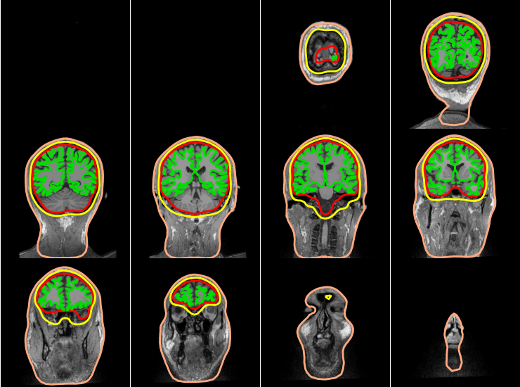
The BEM surfaces are the triangulations of the interfaces between different tissues needed for forward computation. These surfaces are for example the inner skull surface, the outer skull surface and the outer skill surface.

Computing the BEM surfaces requires FreeSurfer and makes use of either of the two following command line tools:

• mne watershed_bem
• mne flash_bem

Here we’ll assume it’s already computed. It takes a few minutes per subject.

For EEG we use 3 layers (inner skull, outer skull, and skin) while for MEG 1 layer (inner skull) is enough.

Let’s look at these surfaces. The function mne.viz.plot_bem() assumes that you have the the bem folder of your subject FreeSurfer reconstruction the necessary files.

mne.viz.plot_bem(subject=subject, subjects_dir=subjects_dir,
                 brain_surfaces='white', orientation='coronal')

Visualization the coregistration¶

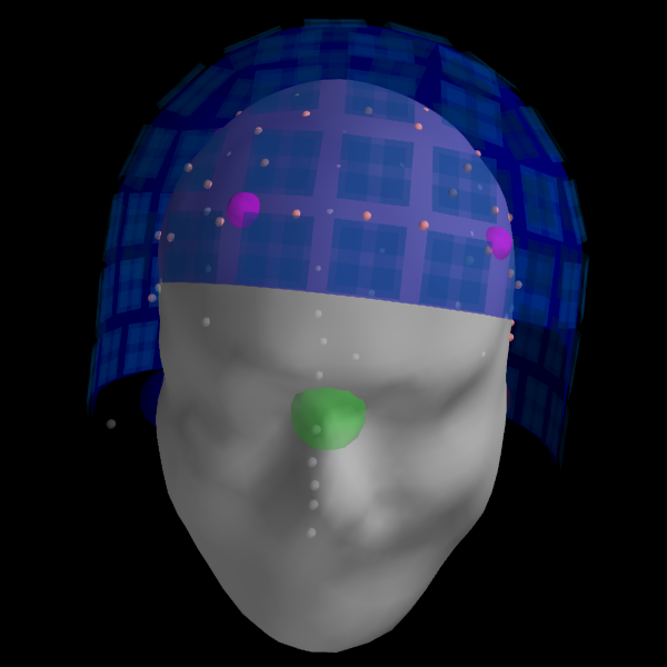
The coregistration is operation that allows to position the head and the sensors in a common coordinate system. In the MNE software the transformation to align the head and the sensors in stored in a so-called trans file. It is a FIF file that ends with -trans.fif. It can be obtained with mne_analyze (Unix tools), mne.gui.coregistration (in Python) or mrilab if you’re using a Neuromag system.

For the Python version see func:mne.gui.coregistration

Here we assume the coregistration is done, so we just visually check the alignment with the following code.

# The transformation file obtained by coregistration
trans = data_path + '/MEG/sample/sample_audvis_raw-trans.fif'

info = mne.io.read_info(raw_fname)
mne.viz.plot_trans(info, trans, subject=subject, dig=True,
                   meg_sensors=True, subjects_dir=subjects_dir)

Compute Source Space¶

The source space defines the position of the candidate source locations. The following code compute such a cortical source space with an OCT-6 resolution.

See Setting up the source space for details on source space definition and spacing parameter.

src = mne.setup_source_space(subject, spacing='oct6',
                             subjects_dir=subjects_dir,
                             add_dist=False, overwrite=True)
print(src)

Out:

Parameters 'fname' and 'overwrite' are deprecated and will be removed in version 0.16. In version 0.15 fname will default to None. Use mne.write_source_spaces instead.
<SourceSpaces: [<surface (lh), n_vertices=155407, n_used=4098, coordinate_frame=MRI (surface RAS)>, <surface (rh), n_vertices=156866, n_used=4098, coordinate_frame=MRI (surface RAS)>]>

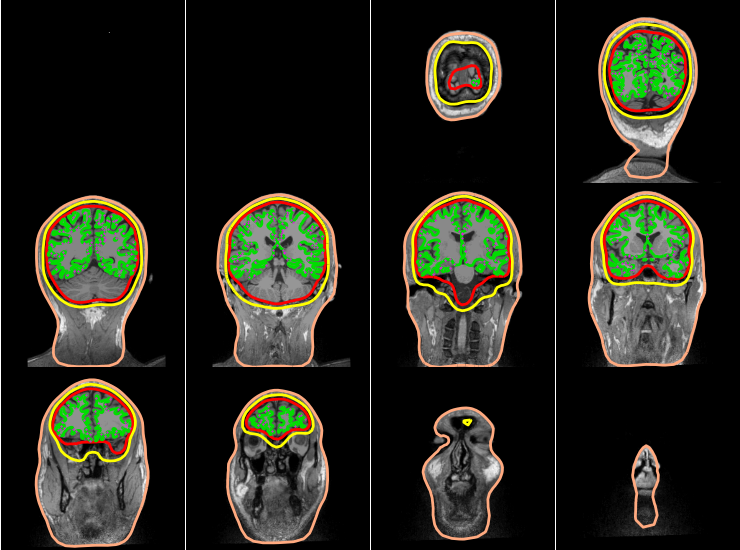
src contains two parts, one for the left hemisphere (4098 locations) and one for the right hemisphere (4098 locations). Sources can be visualized on top of the BEM surfaces.

mne.viz.plot_bem(subject=subject, subjects_dir=subjects_dir,
                 brain_surfaces='white', src=src, orientation='coronal')

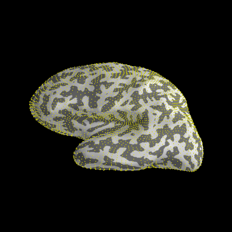
However, only sources that lie in the plotted MRI slices are shown. Let’s write a few lines of mayavi to see all sources.

import numpy as np  # noqa
from mayavi import mlab  # noqa
from surfer import Brain  # noqa

brain = Brain('sample', 'lh', 'inflated', subjects_dir=subjects_dir)
surf = brain._geo

vertidx = np.where(src[0]['inuse'])[0]

mlab.points3d(surf.x[vertidx], surf.y[vertidx],
              surf.z[vertidx], color=(1, 1, 0), scale_factor=1.5)

Compute forward solution¶

We can now compute the forward solution. To reduce computation we’ll just compute a single layer BEM (just inner skull) that can then be used for MEG (not EEG).

We specify if we want a one-layer or a three-layer BEM using the conductivity parameter.

The BEM solution requires a BEM model which describes the geometry of the head the conductivities of the different tissues.

conductivity = (0.3,)  # for single layer
# conductivity = (0.3, 0.006, 0.3)  # for three layers
model = mne.make_bem_model(subject='sample', ico=4,
                           conductivity=conductivity,
                           subjects_dir=subjects_dir)
bem = mne.make_bem_solution(model)

Note that the BEM does not involve any use of the trans file. The BEM only depends on the head geometry and conductivities. It is therefore independent from the MEG data and the head position.

Let’s now compute the forward operator, commonly referred to as the gain or leadfield matrix.

See mne.make_forward_solution() for details on parameters meaning.

fwd = mne.make_forward_solution(raw_fname, trans=trans, src=src, bem=bem,
                                fname=None, meg=True, eeg=False,
                                mindist=5.0, n_jobs=2)
print(fwd)

Out:

<Forward | MEG channels: 306 | EEG channels: 0 | Source space: Surface with 7498 vertices | Source orientation: Free>

We can explore the content of fwd to access the numpy array that contains the gain matrix.

leadfield = fwd['sol']['data']
print("Leadfield size : %d sensors x %d dipoles" % leadfield.shape)

Out:

Leadfield size : 306 sensors x 22494 dipoles

To save to disk a forward solution you can use mne.write_forward_solution() and to read it back from disk mne.read_forward_solution(). Don’t forget that FIF files containing forward solution should end with -fwd.fif.

To get a fixed-orientation forward solution, use mne.convert_forward_solution() to convert the free-orientation solution to (surface-oriented) fixed orientation.

Exercise¶

By looking at Display sensitivity maps for EEG and MEG sensors plot the sensitivity maps for EEG and compare it with the MEG, can you justify the claims that:

• MEG is not sensitive to radial sources
• EEG is more sensitive to deep sources

How will the MEG sensitivity maps and histograms change if you use a free instead if a fixed/surface oriented orientation?

Try this changing the mode parameter in mne.sensitivity_map() accordingly. Why don’t we see any dipoles on the gyri?

Total running time of the script: ( 0 minutes 57.886 seconds)

Generated by Sphinx-Gallery