The aim of this tutorials is to teach you how to compute and apply a linear inverse method such as MNE/dSPM/sLORETA on evoked/raw/epochs data.
import numpy as np
import matplotlib.pyplot as plt

import mne
from mne.datasets import sample
from mne.minimum_norm import (make_inverse_operator, apply_inverse,
                              write_inverse_operator)
Process MEG data
data_path = sample.data_path()
raw_fname = data_path + '/MEG/sample/sample_audvis_filt-0-40_raw.fif'

raw = mne.io.read_raw_fif(raw_fname)
raw.set_eeg_reference()  # set EEG average reference
events = mne.find_events(raw, stim_channel='STI 014')

event_id = dict(aud_r=1)  # event trigger and conditions
tmin = -0.2  # start of each epoch (200ms before the trigger)
tmax = 0.5  # end of each epoch (500ms after the trigger)
raw.info['bads'] = ['MEG 2443', 'EEG 053']
picks = mne.pick_types(raw.info, meg=True, eeg=False, eog=True,
                       exclude='bads')
baseline = (None, 0)  # means from the first instant to t = 0
reject = dict(grad=4000e-13, mag=4e-12, eog=150e-6)

epochs = mne.Epochs(raw, events, event_id, tmin, tmax, proj=True, picks=picks,
                    baseline=baseline, reject=reject)
Out:
Opening raw data file /home/ubuntu/mne_data/MNE-sample-data/MEG/sample/sample_audvis_filt-0-40_raw.fif...
    Read a total of 4 projection items:
        PCA-v1 (1 x 10²)  idle
        PCA-v2 (1 x 10²)  idle
        PCA-v3 (1 x 10²)  idle
        Average EEG reference (1 x 60)  idle
    Range : 6450 ... 48149 =     42.956 ...   320.665 secs
Ready.
Current compensation grade : 0
An average reference projection was already added. The data has been left untouched.
319 events found
Events id: [ 1  2  3  4  5 32]
72 matching events found
Created an SSP operator (subspace dimension = 3)
4 projection items activated
For more details see Computing covariance matrix.
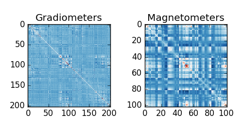
noise_cov = mne.compute_covariance(
    epochs, tmax=0., method=['shrunk', 'empirical'])

fig_cov, fig_spectra = mne.viz.plot_cov(noise_cov, raw.info)

Out:
Loading data for 72 events and 106 original time points ...
    Rejecting  epoch based on EOG : [u'EOG 061']
    Rejecting  epoch based on EOG : [u'EOG 061']
    Rejecting  epoch based on EOG : [u'EOG 061']
    Rejecting  epoch based on EOG : [u'EOG 061']
    Rejecting  epoch based on EOG : [u'EOG 061']
    Rejecting  epoch based on MAG : [u'MEG 1711']
    Rejecting  epoch based on EOG : [u'EOG 061']
    Rejecting  epoch based on EOG : [u'EOG 061']
    Rejecting  epoch based on EOG : [u'EOG 061']
    Rejecting  epoch based on EOG : [u'EOG 061']
    Rejecting  epoch based on EOG : [u'EOG 061']
    Rejecting  epoch based on EOG : [u'EOG 061']
    Rejecting  epoch based on EOG : [u'EOG 061']
    Rejecting  epoch based on EOG : [u'EOG 061']
    Rejecting  epoch based on EOG : [u'EOG 061']
    Rejecting  epoch based on EOG : [u'EOG 061']
    Rejecting  epoch based on EOG : [u'EOG 061']
17 bad epochs dropped
Estimating covariance using SHRUNK
Done.
Estimating covariance using EMPIRICAL
Done.
Using cross-validation to select the best estimator.
Number of samples used : 1705
[done]
Number of samples used : 1705
[done]
log-likelihood on unseen data (descending order):
   shrunk: -1480.993
   empirical: -1628.225
selecting best estimator: shrunk
evoked = epochs.average()
evoked.plot()
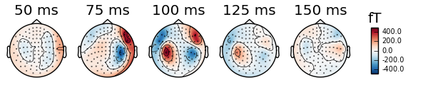
evoked.plot_topomap(times=np.linspace(0.05, 0.15, 5), ch_type='mag')
# Show whitening
evoked.plot_white(noise_cov)


Out:
estimated rank (grad): 203
estimated rank (mag): 102
estimated rank (mag + grad): 305
    Created an SSP operator (subspace dimension = 3)
Setting small MEG eigenvalues to zero.
Not doing PCA for MEG.
# Read the forward solution and compute the inverse operator

fname_fwd = data_path + '/MEG/sample/sample_audvis-meg-oct-6-fwd.fif'
fwd = mne.read_forward_solution(fname_fwd, surf_ori=True)

# Restrict forward solution as necessary for MEG
fwd = mne.pick_types_forward(fwd, meg=True, eeg=False)

# make an MEG inverse operator
info = evoked.info
inverse_operator = make_inverse_operator(info, fwd, noise_cov,
                                         loose=0.2, depth=0.8)

write_inverse_operator('sample_audvis-meg-oct-6-inv.fif',
                       inverse_operator)
Out:
Reading forward solution from /home/ubuntu/mne_data/MNE-sample-data/MEG/sample/sample_audvis-meg-oct-6-fwd.fif...
    Reading a source space...
    Computing patch statistics...
    Patch information added...
    Distance information added...
    [done]
    Reading a source space...
    Computing patch statistics...
    Patch information added...
    Distance information added...
    [done]
    2 source spaces read
    Desired named matrix (kind = 3523) not available
    Read MEG forward solution (7498 sources, 306 channels, free orientations)
    Source spaces transformed to the forward solution coordinate frame
    Converting to surface-based source orientations...
    Average patch normals will be employed in the rotation to the local surface coordinates....
[done]
    306 out of 306 channels remain after picking
Computing inverse operator with 305 channels.
    Created an SSP operator (subspace dimension = 3)
estimated rank (mag + grad): 302
Setting small MEG eigenvalues to zero.
Not doing PCA for MEG.
Total rank is 302
Creating the depth weighting matrix...
    203 planar channels
    limit = 7265/7498 = 10.037795
    scale = 2.52065e-08 exp = 0.8
Computing inverse operator with 305 channels.
Creating the source covariance matrix
Applying loose dipole orientations. Loose value of 0.2.
Whitening the forward solution.
Adjusting source covariance matrix.
Computing SVD of whitened and weighted lead field matrix.
    largest singular value = 4.65276
    scaling factor to adjust the trace = 1.03619e+19
Write inverse operator decomposition in sample_audvis-meg-oct-6-inv.fif...
    Write a source space...
    [done]
    Write a source space...
    [done]
    2 source spaces written
    Writing inverse operator info...
    Writing noise covariance matrix.
    Writing source covariance matrix.
    Writing orientation priors.
    [done]
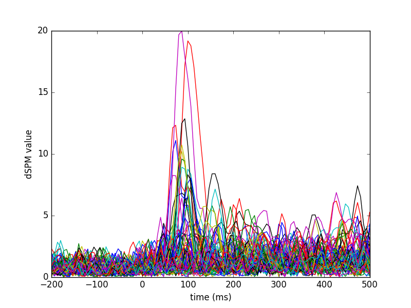
method = "dSPM"
snr = 3.
lambda2 = 1. / snr ** 2
stc = apply_inverse(evoked, inverse_operator, lambda2,
                    method=method, pick_ori=None)

del fwd, inverse_operator, epochs  # to save memory
Out:
Preparing the inverse operator for use...
    Scaled noise and source covariance from nave = 1 to nave = 55
    Created the regularized inverter
    Created an SSP operator (subspace dimension = 3)
    Created the whitener using a full noise covariance matrix (3 small eigenvalues omitted)
    Computing noise-normalization factors (dSPM)...
[done]
Picked 305 channels from the data
Computing inverse...
(eigenleads need to be weighted)...
combining the current components...
(dSPM)...
[done]
View activation time-series
plt.plot(1e3 * stc.times, stc.data[::100, :].T)
plt.xlabel('time (ms)')
plt.ylabel('%s value' % method)
plt.show()
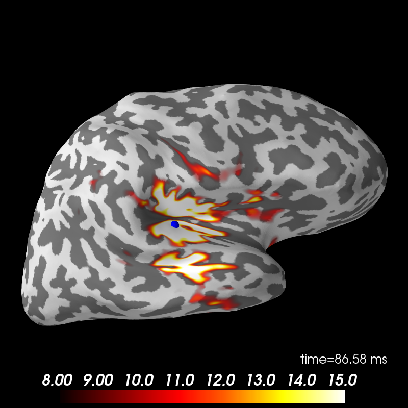
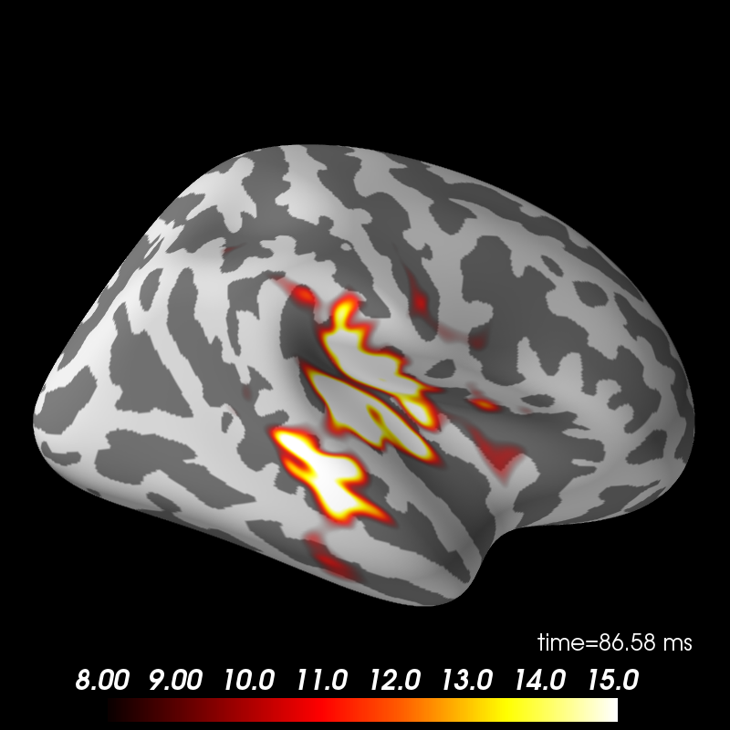
Here we use peak getter to move visualization to the time point of the peak and draw a marker at the maximum peak vertex.
vertno_max, time_max = stc.get_peak(hemi='rh')

subjects_dir = data_path + '/subjects'
brain = stc.plot(surface='inflated', hemi='rh', subjects_dir=subjects_dir,
                 clim=dict(kind='value', lims=[8, 12, 15]),
                 initial_time=time_max, time_unit='s')
brain.add_foci(vertno_max, coords_as_verts=True, hemi='rh', color='blue',
               scale_factor=0.6)
brain.show_view('lateral')
Out:
Updating smoothing matrix, be patient..
Smoothing matrix creation, step 1
Smoothing matrix creation, step 2
Smoothing matrix creation, step 3
Smoothing matrix creation, step 4
Smoothing matrix creation, step 5
Smoothing matrix creation, step 6
Smoothing matrix creation, step 7
Smoothing matrix creation, step 8
Smoothing matrix creation, step 9
Smoothing matrix creation, step 10
colormap: fmin=8.00e+00 fmid=1.20e+01 fmax=1.50e+01 transparent=1
fs_vertices = [np.arange(10242)] * 2
morph_mat = mne.compute_morph_matrix('sample', 'fsaverage', stc.vertices,
                                     fs_vertices, smooth=None,
                                     subjects_dir=subjects_dir)
stc_fsaverage = stc.morph_precomputed('fsaverage', fs_vertices, morph_mat)
brain_fsaverage = stc_fsaverage.plot(surface='inflated', hemi='rh',
                                     subjects_dir=subjects_dir,
                                     clim=dict(kind='value', lims=[8, 12, 15]),
                                     initial_time=time_max, time_unit='s')
brain_fsaverage.show_view('lateral')
Out:
Computing morph matrix...
    Left-hemisphere map read.
    Right-hemisphere map read.
    17 smooth iterations done.
    14 smooth iterations done.
[done]
Updating smoothing matrix, be patient..
Smoothing matrix creation, step 1
Smoothing matrix creation, step 2
Smoothing matrix creation, step 3
Smoothing matrix creation, step 4
Smoothing matrix creation, step 5
Smoothing matrix creation, step 6
Smoothing matrix creation, step 7
Smoothing matrix creation, step 8
Smoothing matrix creation, step 9
Smoothing matrix creation, step 10
colormap: fmin=8.00e+00 fmid=1.20e+01 fmax=1.50e+01 transparent=1
- By changing the method parameter to ‘sloreta’ recompute the source estimates using the sLORETA method.
Total running time of the script: ( 0 minutes 50.241 seconds)