Decoding, a.k.a MVPA or supervised machine learning applied to MEG data in sensor space. Here the classifier is applied to every time point.
import numpy as np
import matplotlib.pyplot as plt

from sklearn.metrics import roc_auc_score
from sklearn.cross_validation import StratifiedKFold

import mne
from mne.datasets import sample
from mne.decoding import TimeDecoding, GeneralizationAcrossTime

data_path = sample.data_path()

plt.close('all')
Set parameters
raw_fname = data_path + '/MEG/sample/sample_audvis_filt-0-40_raw.fif'
event_fname = data_path + '/MEG/sample/sample_audvis_filt-0-40_raw-eve.fif'
tmin, tmax = -0.2, 0.5
event_id = dict(aud_l=1, vis_l=3)

# Setup for reading the raw data
raw = mne.io.read_raw_fif(raw_fname, preload=True)
raw.filter(2, None)  # replace baselining with high-pass
events = mne.read_events(event_fname)

# Set up pick list: EEG + MEG - bad channels (modify to your needs)
raw.info['bads'] += ['MEG 2443', 'EEG 053']  # bads + 2 more
picks = mne.pick_types(raw.info, meg='grad', eeg=False, stim=True, eog=True,
                       exclude='bads')

# Read epochs
epochs = mne.Epochs(raw, events, event_id, tmin, tmax, proj=True,
                    picks=picks, baseline=None, preload=True,
                    reject=dict(grad=4000e-13, eog=150e-6))

epochs_list = [epochs[k] for k in event_id]
mne.epochs.equalize_epoch_counts(epochs_list)
data_picks = mne.pick_types(epochs.info, meg=True, exclude='bads')
Out:
Opening raw data file /home/ubuntu/mne_data/MNE-sample-data/MEG/sample/sample_audvis_filt-0-40_raw.fif...
    Read a total of 4 projection items:
        PCA-v1 (1 x 10²)  idle
        PCA-v2 (1 x 10²)  idle
        PCA-v3 (1 x 10²)  idle
        Average EEG reference (1 x 60)  idle
    Range : 6450 ... 48149 =     42.956 ...   320.665 secs
Ready.
Current compensation grade : 0
Reading 0 ... 41699  =      0.000 ...   277.709 secs...
Setting up high-pass filter at 2 Hz
l_trans_bandwidth chosen to be 2.0 Hz
Filter length of 496 samples (3.303 sec) selected
145 matching events found
4 projection items activated
Loading data for 145 events and 106 original time points ...
    Rejecting  epoch based on EOG : [u'EOG 061']
    Rejecting  epoch based on EOG : [u'EOG 061']
    Rejecting  epoch based on EOG : [u'EOG 061']
    Rejecting  epoch based on EOG : [u'EOG 061']
    Rejecting  epoch based on EOG : [u'EOG 061']
    Rejecting  epoch based on EOG : [u'EOG 061']
    Rejecting  epoch based on EOG : [u'EOG 061']
    Rejecting  epoch based on EOG : [u'EOG 061']
    Rejecting  epoch based on EOG : [u'EOG 061']
    Rejecting  epoch based on EOG : [u'EOG 061']
    Rejecting  epoch based on EOG : [u'EOG 061']
    Rejecting  epoch based on EOG : [u'EOG 061']
    Rejecting  epoch based on EOG : [u'EOG 061']
    Rejecting  epoch based on EOG : [u'EOG 061']
    Rejecting  epoch based on EOG : [u'EOG 061']
    Rejecting  epoch based on EOG : [u'EOG 061']
    Rejecting  epoch based on EOG : [u'EOG 061']
    Rejecting  epoch based on EOG : [u'EOG 061']
    Rejecting  epoch based on EOG : [u'EOG 061']
    Rejecting  epoch based on EOG : [u'EOG 061']
    Rejecting  epoch based on EOG : [u'EOG 061']
    Rejecting  epoch based on EOG : [u'EOG 061']
22 bad epochs dropped
Dropped 11 epochs
Dropped 0 epochs
We’ll use the default classifer for a binary classification problem which is a linear Support Vector Machine (SVM).
td = TimeDecoding(predict_mode='cross-validation', n_jobs=1)

# Fit
td.fit(epochs)

# Compute accuracy
td.score(epochs)

# Plot scores across time
td.plot(title='Sensor space decoding')
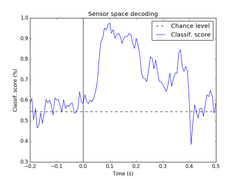
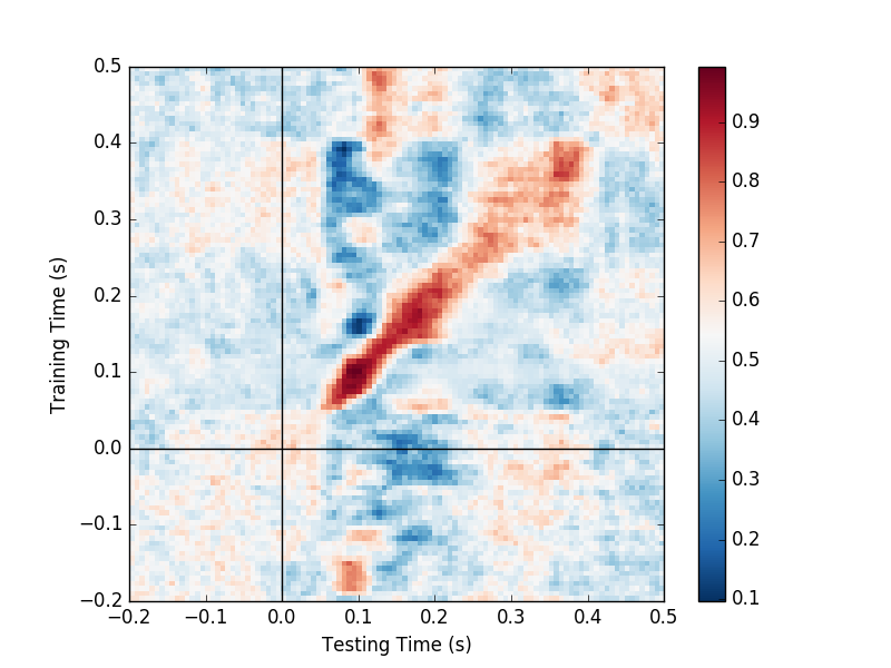
This runs the analysis used in [1] and further detailed in [2]
Here we’ll use a stratified cross-validation scheme.
# make response vector
y = np.zeros(len(epochs.events), dtype=int)
y[epochs.events[:, 2] == 3] = 1
cv = StratifiedKFold(y=y)  # do a stratified cross-validation

# define the GeneralizationAcrossTime object
gat = GeneralizationAcrossTime(predict_mode='cross-validation', n_jobs=1,
                               cv=cv, scorer=roc_auc_score)

# fit and score
gat.fit(epochs, y=y)
gat.score(epochs)

# let's visualize now
gat.plot()
gat.plot_diagonal()

- Can you improve the performance using full epochs and a common spatial pattern (CSP) used by most BCI systems?
- Explore other datasets from MNE (e.g. Face dataset from SPM to predict Face vs. Scrambled)
Have a look at the example Decoding in sensor space data using the Common Spatial Pattern (CSP)
| [1] | Jean-Remi King, Alexandre Gramfort, Aaron Schurger, Lionel Naccache and Stanislas Dehaene, “Two distinct dynamic modes subtend the detection of unexpected sounds”, PLOS ONE, 2013, http://www.ncbi.nlm.nih.gov/pubmed/24475052 |
| [2] | King & Dehaene (2014) ‘Characterizing the dynamics of mental representations: the temporal generalization method’, Trends In Cognitive Sciences, 18(4), 203-210. http://www.ncbi.nlm.nih.gov/pubmed/24593982 |
Total running time of the script: ( 0 minutes 24.523 seconds)