import os.path as op
import numpy as np

import mne

data_path = op.join(mne.datasets.sample.data_path(), 'MEG', 'sample')
raw = mne.io.read_raw_fif(op.join(data_path, 'sample_audvis_raw.fif'))
raw.set_eeg_reference()  # set EEG average reference
events = mne.read_events(op.join(data_path, 'sample_audvis_raw-eve.fif'))
Out:
Opening raw data file /home/ubuntu/mne_data/MNE-sample-data/MEG/sample/sample_audvis_raw.fif...
    Read a total of 3 projection items:
        PCA-v1 (1 x 10²)  idle
        PCA-v2 (1 x 10²)  idle
        PCA-v3 (1 x 10²)  idle
    Range : 25800 ... 192599 =     42.956 ...   320.670 secs
Ready.
Current compensation grade : 0
Adding average EEG reference projection.
1 projection items deactivated
The visualization module (mne.viz) contains all the plotting functions
that work in combination with MNE data structures. Usually the easiest way to
use them is to call a method of the data container. All of the plotting
method names start with plot. If you’re using Ipython console, you can
just write raw.plot and ask the interpreter for suggestions with a
tab key.
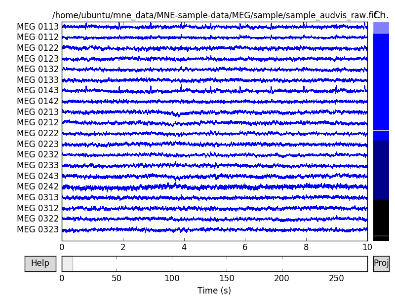
To visually inspect your raw data, you can use the python equivalent of
mne_browse_raw.
raw.plot(block=True)
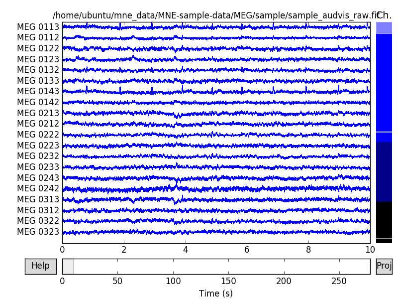
The channels are color coded by channel type. Generally MEG channels are
colored in different shades of blue, whereas EEG channels are black. The
scrollbar on right side of the browser window also tells us that two of the
channels are marked as bad. Bad channels are color coded gray. By
clicking the lines or channel names on the left, you can mark or unmark a bad
channel interactively. You can use +/- keys to adjust the scale (also = works
for magnifying the data). Note that the initial scaling factors can be set
with parameter scalings. If you don’t know the scaling factor for
channels, you can automatically set them by passing scalings=’auto’. With
pageup/pagedown and home/end keys you can adjust the amount of data
viewed at once.
You can enter annotation mode by pressing a key. In annotation mode you
can mark segments of data (and modify existing annotations) with the left
mouse button. You can use the description of any existing annotation or
create a new description by typing when the annotation dialog is active.
Notice that the description starting with the keyword 'bad' means that
the segment will be discarded when epoching the data. Existing annotations
can be deleted with the right mouse button. Annotation mode is exited by
pressing a again or closing the annotation window. See also
mne.Annotations and Marking bad raw segments with annotations. To see all the
interactive features, hit ? key or click help in the lower left
corner of the browser window.
Warning
Annotations are modified in-place immediately at run-time. Deleted annotations cannot be retrieved after deletion.
The channels are sorted by channel type by default. You can use the order
parameter of raw.plot to group the channels in a
different way. order='selection' uses the same channel groups as MNE-C’s
mne_browse_raw (see Selection). The selections are defined in
mne-python/mne/data/mne_analyze.sel and by modifying the channels there,
you can define your own selection groups. Notice that this also affects the
selections returned by mne.read_selection(). By default the selections
only work for Neuromag data, but order='position' tries to mimic this
behavior for any data with sensor positions available. The channels are
grouped by sensor positions to 8 evenly sized regions. Notice that for this
to work effectively, all the data channels in the channel array must be
present. The order parameter can also be passed as an array of ints
(picks) to plot the channels in the given order.
raw.plot(order='selection')
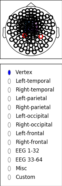
We read the events from a file and passed it as a parameter when calling the method. The events are plotted as vertical lines so you can see how they align with the raw data.
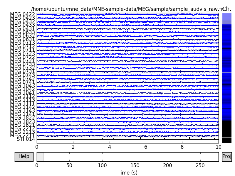
We can check where the channels reside with plot_sensors. Notice that
this method (along with many other MNE plotting functions) is callable using
any MNE data container where the channel information is available.
raw.plot_sensors(kind='3d', ch_type='mag', ch_groups='position')
We used ch_groups='position' to color code the different regions. It uses
the same algorithm for dividing the regions as order='position' of
raw.plot. You can also pass a list of picks to
color any channel group with different colors.
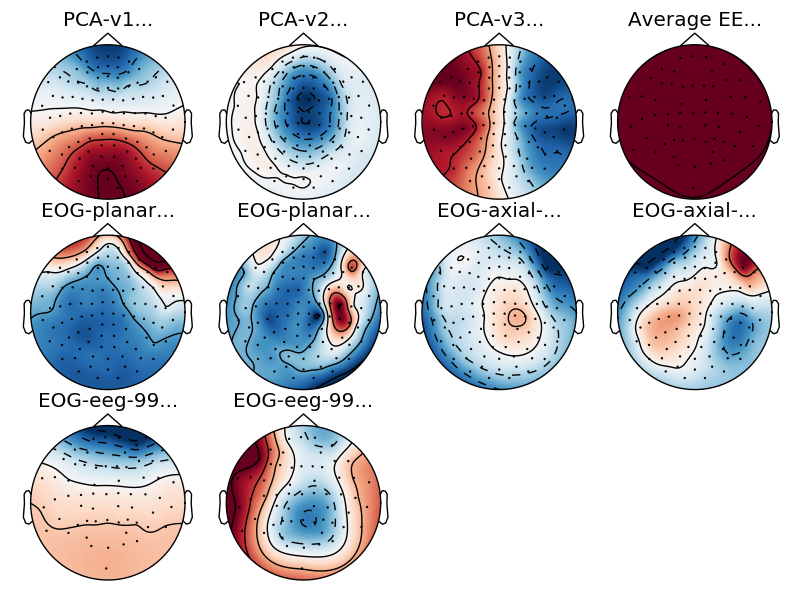
Now let’s add some ssp projectors to the raw data. Here we read them from a file and plot them.
projs = mne.read_proj(op.join(data_path, 'sample_audvis_eog-proj.fif'))
raw.add_proj(projs)
raw.plot_projs_topomap()
Out:
Read a total of 6 projection items:
        EOG-planar-998--0.200-0.200-PCA-01 (1 x 203)  idle
        EOG-planar-998--0.200-0.200-PCA-02 (1 x 203)  idle
        EOG-axial-998--0.200-0.200-PCA-01 (1 x 10²)  idle
        EOG-axial-998--0.200-0.200-PCA-02 (1 x 10²)  idle
        EOG-eeg-998--0.200-0.200-PCA-01 (1 x 59)  idle
        EOG-eeg-998--0.200-0.200-PCA-02 (1 x 59)  idle
6 projection items deactivated
The first three projectors that we see are the SSP vectors from empty room measurements to compensate for the noise. The fourth one is the average EEG reference. These are already applied to the data and can no longer be removed. The next six are the EOG projections that we added. Every data channel type has two projection vectors each. Let’s try the raw browser again.
raw.plot()
Now click the proj button at the lower right corner of the browser
window. A selection dialog should appear, where you can toggle the projectors
on and off. Notice that the first four are already applied to the data and
toggling them does not change the data. However the newly added projectors
modify the data to get rid of the EOG artifacts. Note that toggling the
projectors here doesn’t actually modify the data. This is purely for visually
inspecting the effect. See mne.io.Raw.del_proj() to actually remove the
projectors.
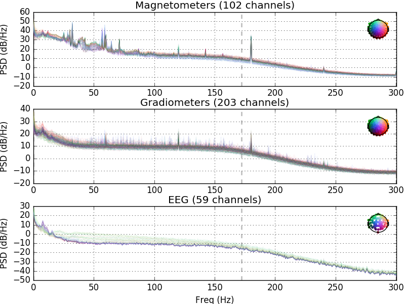
Raw container also lets us easily plot the power spectra over the raw data. Here we plot the data using spatial_colors to map the line colors to channel locations (default in versions >= 0.15.0). Other option is to use the average (default in < 0.15.0). See the API documentation for more info.
raw.plot_psd(tmax=np.inf, average=False)
Out:
Effective window size : 3.410 (s)
Effective window size : 3.410 (s)
Effective window size : 3.410 (s)
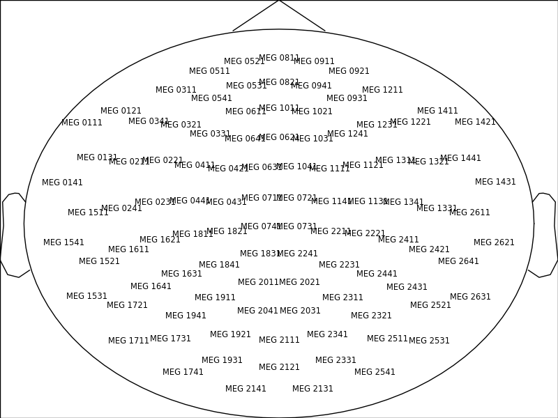
Plotting channel-wise power spectra is just as easy. The layout is inferred from the data by default when plotting topo plots. This works for most data, but it is also possible to define the layouts by hand. Here we select a layout with only magnetometer channels and plot it. Then we plot the channel wise spectra of first 30 seconds of the data.
layout = mne.channels.read_layout('Vectorview-mag')
layout.plot()
raw.plot_psd_topo(tmax=30., fmin=5., fmax=60., n_fft=1024, layout=layout)

Out:
Effective window size : 1.705 (s)
Total running time of the script: ( 0 minutes 21.698 seconds)