![]()
Contents
The raw data processor mne_browse_raw is designed for simple raw data viewing and processing operations. In addition, the program is capable of off-line averaging and estimation of covariance matrices. mne_browse_raw can be also used to view averaged data in the topographical layout. Finally, mne_browse_raw can communicate with mne_analyze described in Interactive analysis with mne_analyze to calculate current estimates from raw data interactively.
mne_browse_raw has also an alias, mne_process_raw. If mne_process_raw is invoked, no user interface appears. Instead, command line options are used to specify the filtering parameters as well as averaging and covariance-matrix estimation command files for batch processing. This chapter discusses both mne_browse_raw and mne_process_raw.
See command-line documentation of mne_browse_raw and mne_process_raw.
The user interface of mne_browse_raw
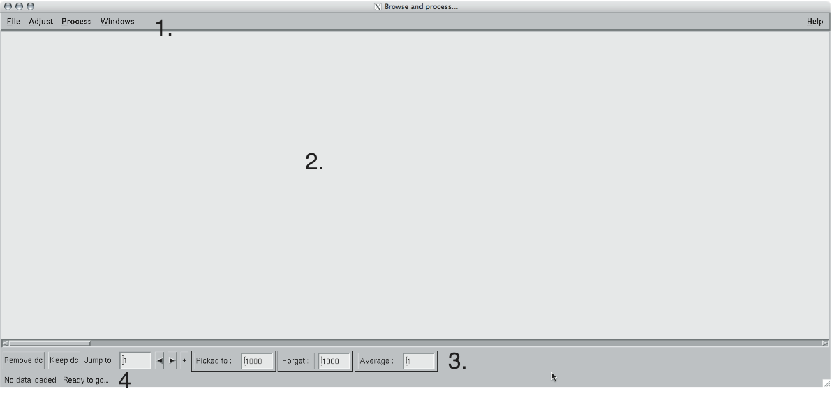
The mne_browse_raw user interface contains the following areas:
The viewing and averaging tools allow quick browsing of the raw data with triggers, adding new triggers, and averaging on a single trigger.
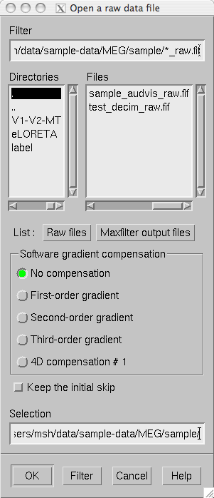
Selecting Open from file menu pops up the dialog shown in The Open dialog..
The Raw files and Maxfilter output buttons change the file name filter to include
names which end with _raw.fif or sss.fif ,
respectively, to facilitate selection of original raw files or those
processed with the Neuromag Maxfilter (TM) software
The options under Software gradient compensation allow selection of the compensation grade for the data. These selections apply to the CTF data only. The standard choices are No compensation and Third-order gradient. If other than No compensation is attempted for non-CTF data, an error will be issued. The compensation selection affects the averages and noise-covariance matrices subsequently computed. The desired compensation takes effect independent of the compensation state of the data in the file, i.e., already compensated data can be uncompensated and vice versa. For more information on software gradient compensation please consult Applying software gradient compensation.
The Keep the initial skip button controls how the initial segment of data not stored in the raw data file is handled. During the MEG acquisition data are collected continuously but saving to the raw data file is controlled by the Record raw button. Initial skip refers to the segment of data between the start of the recording and the first activation of Record raw . If Keep initial skip is set, this empty segment is taken into account in timing, otherwise time zero is set to the beginning of the data stored to disk.
When a raw data file is opened, the digital trigger channel is scanned for events. For large files this may take a while.
Note
After scanning the trigger channel for events, mne_browse_raw and mne_process_raw produce a fif file containing the event information. This file will be called <raw data file name without fif extension> -eve.fif . If the same raw data file is opened again, this file will be consulted for event information thus making it unnecessary to scan through the file for trigger line events.
Note
You can produce the fif event file by running mne_process_raw as follows: mne_process_raw --raw <raw data file> . The fif format event files can be read and written with the mne_read_events and mne_write_events functions in the MNE Matlab toolbox, see Matlab toolbox.
The Open dialog.
This menu item brings up a standard file selection dialog to load evoked-response data from files. All data sets from a file are loaded automatically and display in the average view window, see Topographical data displays. The data loaded are affected by the scale settings, see, Scales, the filter, see Filter, and the options selected in the Manage averages dialog, see Managing averages.
It is possible to save filtered and projected data into a new raw data file. When you invoke the save option from the file menu, you will be prompted for the output file name and a down-sampling factor. The sampling frequency after down-sampling must be at least three times the lowpass filter corner frequency. The output will be split into files which are just below 2 GB so that the fif file maximum size is not exceed.
If <filename> ends
with .fif or _raw.fif , these endings are
deleted. After these modifications, _raw.fif is inserted
after the remaining part of the file name. If the file is split
into multiple parts, the additional parts will be called <name> - <number> _raw.fif .
For downsampling and saving options in mne_process_raw ,
see mne_process_raw.
Brings up a file selection dialog which allows changing of the working directory.
Selecting Read projection… from the File menu, pops up a dialog to enter a name of a file containing a signal-space projection operator to be applied to the data. There is an option to keep existing projection items.
Note
Whenever EEG channels are present in the data, a projection item corresponding to the average EEG reference is automatically added.
The Save projection… item in the File menu pops up a dialog to save the present projection operator into a file. Normally, the EEG average reference projection is not included. If you want to include it, mark the Include EEG average reference option. If your MEG projection includes items for both magnetometers and gradiometers and you want to use the projection operator file output from here in the Neuromag Signal processor (graph) software, mark the Enforce compatibility with graph option.
Applies the current selection of bad channels to the currently open raw file.
Reads a text format event file. For more information on events, see Events and annotations.
Reads a fif format event file. For more information on events, see Events and annotations.
Brings up a a dialog to save all or selected types of events into a text file. This file can be edited and used in the averaging and covariance matrix estimation as an input file to specify the time points of events, see Event files. For more information on events, see Events and annotations.
Save the events in fif format. These binary event files can be read and written with the mne_read_events and mne_write_events functions in the MNE Matlab toolbox, see Matlab toolbox. For more information on events, see Events and annotations.
This menu choice allows loading of channel derivation data files created with the mne_make_derivations utility, see mne_make_derivations, or using the interactive derivations editor in mne_browse_raw , see Derivations, Most common use of derivations is to calculate differences between EEG channels, i.e., bipolar EEG data. Since any number of channels can be included in a derivation with arbitrary weights, other applications are possible as well. Before a derivation is accepted to use, the following criteria have to be met:
Multiple derivation data files can be loaded by specifying the Keep previous derivations option in the dialog that specifies the derivation file to be loaded. After a derivation file has been successfully loaded, a list of available derivations will be shown in a message dialog.
Each of the derived channels has a name specified when the derivation file was created. The derived channels can be included in channel selections, see Selection. At present, derived channels cannot be displayed in topographical data displays. Derived channels are not included in averages or noise covariance matrix estimation.
Note
If the file $HOME/.mne/mne_browse_raw-deriv.fif exists and contains derivation data, it is loaded automatically when mne_browse_raw starts unless the --deriv option has been used to specify a nonstandard derivation file, see mne_browse_raw.
Saves the current derivations into a file.
This choice loads a new set of channel selections. The default directory for the selections is $HOME/.mne. If this directory does not exist, it will be created before bringing up the file selection dialog to load the selections.
This choice brings up a dialog to save the current channel selections. This is particularly useful if the standard set of selections has been modified as explained in Selection. The default directory for the selections is $HOME/.mne. If this directory does not exist, it will be created before bringing up the file selection dialog to save the selections. Note that all currently existing selections will be saved, not just those added to the ones initially loaded.
Selecting Filter… from the Adjust menu pops up the dialog shown in The filter adjustment dialog..

The filter adjustment dialog.
The items in the dialog have the following functions:
Highpass (Hz)
The half-amplitude point of the highpass filter. The width of the transition from zero to one can be specified with the--highpasswcommand-line option, see mne_browse_raw. Lowest feasible highpass value is constrained by the length of the filter and sampling frequency. You will be informed when you press OK or Apply if the selected highpass could not be realized. The default value zero means no highpass filter is applied in addition to the analog highpass present in the data.
Lowpass (Hz)
The half-amplitude point of the lowpass filter.
Lowpass transition (Hz)
The width of the \(\cos^2\)-shaped transition from one to zero, centered at the Lowpass value.
Filter active
Selects whether or not the filter is applied to the data.
The filter is realized in the frequency domain and has a zero phase shift. When a filter is in effect, the value of the first sample in the file is subtracted from the data to correct for an initial dc offset. This procedure also eliminates any filter artifacts in the beginning of the data.
Note
The filter affects both the raw data and evoked-response data loaded from files. However, the averages computed in mne_browse_raw and shown in the topographical display are not refiltered if the filter is changed after the average was computed.
Selecting Scales… from the Adjust menu pops up the dialog shown in The Scales dialog..
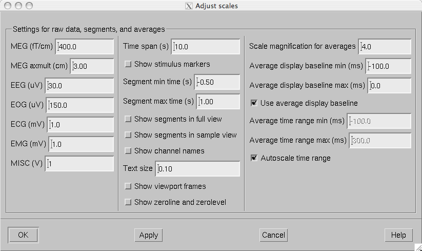
The Scales dialog.
The items in the dialog have the following functions:
MEG (fT/cm)
Sets the scale for MEG planar gradiometer channels in fT/cm. All scale values are defined from zero to maximum, i.e., the viewport where signals are plotted in have the limits ± <scale value> .
MEG axmult (cm)
The scale for MEG magnetometers and axial gradiometers is defined by multiplying the gradiometer scale by this number, yielding units of fT.
EEG (\(\mu V\))
The scale for EEG channels in \(\mu V\).
EOG (\(\mu V\))
The scale for EOG channels in \(\mu V\).
ECG (mV)
The scale for ECG channels in mV.
EMG (mV)
The scale for EMG channels in mV.
MISC (V)
The scale for MISC channels in V.
Time span (s)
The length of raw data displayed in the main window at a time.
Show stimulus markers
Draw vertical lines at time points where the digital trigger channel has a transition from zero to a nonzero value.
Segment min. time (s)
It is possible to show data segments in the topographical (full view) layout, see below. This parameter sets the starting time point, relative to the selected time, to be displayed.
Segment max. time (s)
This parameter sets the ending time point, relative to the current time, to be displayed in the topographical layout.
Show segments in full view
Switches on the display of data segments in the topographical layout.
Show segments in sample view
Switches on the display of data segments in a “sidebar” to the right of the main display.
Show channel names
Show the names of the channels in the topographical displays.
Text size
Size of the channel number text as a fraction of the height of each viewport.
Show viewport frames
Show the boundaries of the viewports in the topographical displays.
Show zeroline and zerolevel
Show the zero level, i.e., the baseline level in the topographical displays. In addition, the zero time point is indicated in the average views if it falls to the time range, i.e., if the minimum of the time scale is negative and the maximum is positive.
Scale magnification for averages
For average displays, the scales are made more sensitive by this factor.
Average display baseline min (ms)
Sets the lower time limit for the average display baseline. This setting does not affect the averages stored.
Average display baseline max (ms)
Sets the upper time limit for the average display baseline. This setting does not affect the averages stored.
Use average display baseline
Switches the application of a baseline to the displayed averages on and off.
Average time range min (ms)
Sets the minimum time for the average display. This setting is inactive if Autoscale time range is on.
Average time range max (ms)
Sets the maximum time for the average data display. This setting is inactive if Autoscale time range is on.
Autoscale time range
Set the average display time range automatically to be long enough to accommodate all data.
Brings up the interactive derivations editor. This editor can be used to add or modify derived channels, i.e., linear combinations of signals actually recorded. Channel derivations can be also created and modified using the mne_make_derivations tool, see mne_make_derivations. The interactive editor contains two main areas:
The Define button interprets the arithmetic expressions in the text area as new derivations and closes the dialog. The Cancel button closes the dialog without any change in the derivations.
Recommended workflow for defining derived EEG channels and associated selections interactively involves the following steps:
--revert option.$HOME/.mne/mne_browse_raw-deriv.fif ).$HOME/.mne/mne_browse_raw.sel .Brings up a dialog to select channels to be shown in the main raw data display. This dialog also allows modification of the set of channel selections as described below.
By default, the available selections are defined by the file $MNE_ROOT/share/mne/mne_browse_raw/mne_browse_raw.sel .
This default channel selection file can be modified by copying the
file into $HOME/.mne/mne_browse_raw.sel . The format
of this text file should be self explanatory.
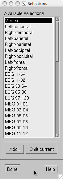
The channel selection dialog.
The channel selection dialog is shown in The channel selection dialog.. The number of items in the selection list depends on the contents of your selection file. If the list has the keyboard focus you can easily move from one selection to another with the up and down arrow keys.
The two buttons below the channel selection buttons facilitate the modification of the selections:
Add…
Brings up the selection dialog shown in Dialog to create a new channel selection. to create new channel selections.
Omit current
Delete the current channel selection. Deletion only affects the selections in the memory of the program. To save the changes permanently into a file, use Save channel selections… in the File menu, see Save channel selections.
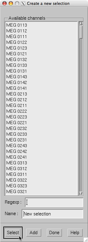
Dialog to create a new channel selection.
The components of the selection creation dialog shown in Dialog to create a new channel selection. have the following functions:
List of channel names
The channels selected from this list will be included in the new channel selection. A selection can be extended with the control key. A range of channels can be selected with the shift key. The list contains both the original channels actually present in the file and the names of the channels in currently loaded derivation data, see Load derivations.
Regexp:
This provides another way to select channels. By entering here a regular expression as defined in IEEE Standard 1003.2 (POSIX.2), all channels matching it will be selected and added to the present selection. An empty expression deselects all items in the channel list. Some useful regular expressions are listed in Examples of regular expressions for channel selections. In the present version, regular matching does not look at the derived channels.
Name:
This text field specifies the name of the new selection.
Select
Select the channels specified by the regular expression. The same effect can be achieved by entering return in the Regexp: .
Add
Add a new channel selection which contains the channels selected from the channel name list. The name of the selection is specified with the Name: text field.
| Regular expression | Meaning |
|---|---|
MEG |
Selects all MEG channels. |
EEG |
Selects all EEG channels. |
MEG.*1$ |
Selects all MEG channels whose names end with the number 1, i.e., all magnetometer channels. |
MEG.*[2,3]$ |
Selects all MEG gradiometer channels. |
EEG|STI 014 |
Selects all EEG channels and stimulus channel STI 014. |
^M |
Selects all channels whose names begin with the letter M. |
Note
The interactive tool for creating the channel selections does not allow you to change the order of the selected channels from that given by the list of channels. However, the ordering can be easily changed by manually editing the channel selection file in a text editor.
Shows a selection of available layouts for the topographical
views (full view and average display). The system-wide layout files
reside in $MNE_ROOT/share/mne/mne_analyze/lout . In
addition any layout files residing in $HOME/.mne/lout are
listed. The default layout is Vectorview-grad. If there is a layout
file in the user’s private layout directory ending with -default.lout ,
that layout will be used as the default instead. The Default button
returns to the default layout.
The format of the layout files is:
<plot area limits><viewport definition #1>…<viewport definition #N>
The <plot area limits> define the size of the plot area (\(x_{min}\ x_{max}\ y_{min}\ y_{max}\)) which should accommodate all view ports. When the layout is used, the plot area will preserve its aspect ratio; if the plot window has a different aspect ratio, there will be empty space on the sides.
The viewports define the locations of the individual channels in the plot. Each viewport definition consists of
<number> \(x_0\ y_0\) <width> <height> <name> [: <name> ] …
where number is a viewport number (not used by the MNE software), \(x_0\) and \(y_0\) are the coordinates of the lower-left corner of the viewport, <width> and <height> are the viewport dimensions, and <name> is a name of a channel. Multiple channel names can be specified by separating them with a colon.
When a measurement channel name is matched to a layout channel name, all spaces are removed from the channel names and the both the layout channel name and the data channel name are converted to lower case. In addition anything including and after a hyphen (-) is omitted. The latter convention facilitates using CTF MEG system data, which has the serial number of the system appended to the channel name with a dash. Removal of the spaces is important for the Neuromag Vectorview data because newer systems do not have spaces in the channel names like the original Vectorview systems did.
Note
The mne_make_eeg_layout utility can be employed to create a layout file matching the positioning of EEG electrodes, see mne_make_eeg_layout.
Lists the currently available signal-space projection (SSP) vectors and allows the activation and deactivation of items. For more information on SSP, see The Signal-Space Projection (SSP) method.
Brings up a dialog to select software gradient compensation. This overrides the choice made at the open time. For details, see Open, above.
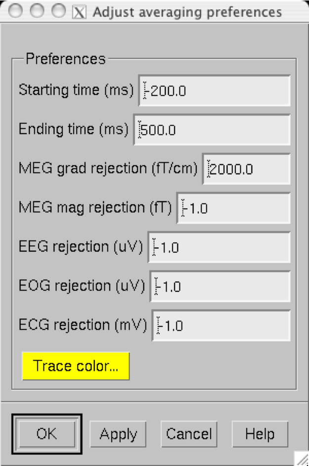
Averaging preferences.
Selecting Averaging preferences… from the Adjust menu pops up the dialog shown in Averaging preferences.. These settings apply only to the simple averages calculated with help of tools residing just below the main raw data display, see The tool bar. These settings are also applied when a covariance matrix is computed to create a SSP operator as described in Creating a new SSP operator and in the computation of a covariance matrix from raw data, see Estimation of a covariance matrix from raw data.
The items in the dialog have the following functions:
Starting time (ms)
Beginning time of the epoch to be averaged (relative to the trigger).
Ending time (ms)
Ending time of the epoch to be averaged.
Ignore around stimulus (ms)
Ignore this many milliseconds on both sides of the trigger when considering the epoch. This parameter is useful for ignoring large stimulus artefacts, e.g., from electrical somatosensory stimulation.
MEG grad rejection (fT/cm)
Rejection criterion for MEG planar gradiometers. If the peak-to-peak value of any planar gradiometer epoch exceed this value, it will be omitted. A negative value turns off rejection for a particular channel type.
MEG mag rejection (fT)
Rejection criterion for MEG magnetometers and axial gradiometers.
EEG rejection (\(\mu V\))
Rejection criterion for EEG channels.
EOG rejection (\(\mu V\))
Rejection criterion for EOG channels.
ECG rejection (mV)
Rejection criterion for ECG channels.
MEG grad no signal (fT/cm)
Signal detection criterion for MEG planar gradiometers. The peak-to-peak value of all planar gradiometer signals must exceed this value, for the epoch to be included. This criterion allows rejection of data with saturated or otherwise dysfunctional channels.
MEG mag no signal (fT)
Signal detection criterion for MEG magnetometers and axial gradiometers.
EEG no signal (\(\mu V\))
Signal detection criterion for EEG channels.
EOG no signal (\(\mu V\))
Signal detection criterion for EOG channels.
ECG no signal (mV)
Signal detection criterion for ECG channels.
Fix trigger skew
This option has the same effect as the FixSkew parameter in averaging description files, see Common parameters.
Trace color
The color assigned for the averaged traces in the display can be adjusted by pressing this button.
The Average… menu item pops up a file selection dialog to access a description file for batch-mode averaging. The structure of these files is described in Description files for off-line averaging. All parameters for the averaging are taken from the description file, i.e., the parameters set in the averaging preferences dialog (Averaging preferences) do not effect the result.
The Compute covariance… menu item pops up a file selection dialog to access a description file which specifies the options for the estimation of a covariance matrix. The structure of these files is described in Description files for covariance matrix estimation.
The Compute raw data covariance… menu item pops up a dialog which specifies a time range for raw data covariance matrix estimation and the file to hold the result. If a covariance matrix is computed in this way, the rejection parameters specified in averaging preferences are in effect. For description of the rejection parameters, see Averaging preferences. The time range can be also selected interactively from the main raw data display by doing a range selection with shift left button drag.
The Create a new SSP operator… menu choice computes a new SSP operator as discussed in Estimation of the noise subspace.
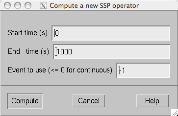
Time range specification for SSP operator calculation
When Create a new SSP operator… selected, a window shown in Time range specification for SSP operator calculation is popped up. It allows the specification of a time range to be employed in the calculation of a raw data covariance matrix. The time range can be also selected interactively from the main raw data display by doing a range selection with shift left button drag. Normally, you should use empty room data for this computation. For the estimation of the covariance matrix any existing projection will be temporarily switched off. Remember to inspect your data for bad channels and select an appropriate filter setting before creating a new SSP operator. The artifact rejection parameters specified averaging preferences will be applied in the covariance matrix calculation, see Averaging preferences.
Instead of using continuous raw data, it is also possible to employ short epochs around triggers (events) in the calculation of the new SSP operator by specifying a positive event number in the time specification dialog. This option is very useful, e.g., to remove MCG/ECG artifacts from the data to facilitate detection of epileptic spikes:
Once the parameters are set, click Compute to calculate a covariance matrix according to you your specifications. Once the covariance matrix is ready, the parts corresponding to magnetometer or axial gradiometer, planar gradiometer, and EEG channels are separated and the corresponding eigenvectors and eigenvalues are computed. Once complete, a projection selector with eight magnetometer eigenvectors, five planar gradiometer eigenvectors, three EEG eigenvectors, as well as the existing projection items is displayed.
Using the projection selector, you can experiment which vectors have a significant effect on the noise level of the data. You should strive for using a minimal number of vectors. When the selection is complete, you can click Accept to introduce this selection of vectors as the new projection operator. Discard abandons the set of calculated vectors. Whenever EEG channels are present in the data, a projection item corresponding to the average EEG reference is automatically added when a new projection operator is introduced. More information on the SSP method can be found in The Signal-Space Projection (SSP) method.
Note
The new projection data created in mne_browse_raw is not automatically copied to the data file. You need to create a standalone projection file from File/Save projection… to save the new projection data and load it manually after the data file has been loaded if you want to include in any subsequent analysis.
Note
The command-line options for mne_process_raw allow calculation of the SSP operator from continuous data in the batch mode, see mne_process_raw.
The contents of the Help menu is shown in The Help menu.:
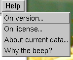
The Help menu.
On version…
Displays the version and compilation date of the program.
On license…
Displays the license information.
About current data…
Displays essential information about the currently loaded data set.
Why the beep?
In some simple error situations, mne_browse_raw does not pop up an error dialog but refuses the action and rings the bell. The reason for this can be displayed through this help menu item.
The main data displays shows a section of the raw data in a strip-chart recorder format. The names of the channels displayed are shown on the left. The selection of channels is controlled from the selection dialog, see Selection. The length of the data section displayed is controlled from the scales dialog (Scales) and the filtering from the filter dialog (Filter). A signal-space projection can be applied to the data by loading a projection operator (Read projection). The selection of the projection operator items is controlled from the projection dialog described in Projection.
The control and browsing functions of the main data display are:
Selection of bad channels
If you click on a channel name the corresponding channel is marked bad or reinstated as an acceptable one. A channel marked bad is not considered in the artefact rejection procedures in averaging and it is omitted from the signal-space projection operations.
Browsing
Browsing through the data. The section of data displayed can be selected from the scroll bar at the bottom of the display. Additional browsing functionality will be discussed n In addition, if the strip-chart display has the keyboard focus, you can scroll back and forth with the page up and page down keys.
Selection of time points
When you click on the data with the left button, a vertical marker appears. If Show segments in full view and/or Show segments in sample view is active in the scales dialog (see Scales), a display of an epoch of data specified in the scales dialog will appear. For more information on full view, see Topographical data displays. Multiple time points can be selected by holding the control key down when clicking. If multiple time points are selected several samples will be shown in the sample and/or full view, aligned at the picked time point. The tool bar offers functions to operate on the selected time points, see The tool bar.
Range selection
Range selection. If you drag on the signals with the left mouse button and the shift key down, a range of times will be selected and displayed in the sample and/or full view. Note: All previous selections are cleared by this operation.
Saving a copy of the display
The right mouse button invokes a popup menu which allows saving of the display in various formats. Best quality is achieved with the Illustrator format. This format has the benefit that it is object oriented and can be edited in Adobe Illustrator.
Drag and drop
Graphics can be moved to one of the Elekta-Neuromag report composer (cliplab ) view areas with the middle mouse button.
Note
When selecting bad channels, switch the signal-space projection off from the projection dialog. Otherwise bad channels may not be easily recognizable.
Note
The cliplab drag-and-drop functionality requires that you have the proprietary Elekta-Neuromag analysis software installed. mne_browse_raw is compatible with cliplab versions 1.2.13 and later.
If the strip-chart display has the input focus (click on it, if you are unsure) the keyboard and mouse can be used to browse the data as follows:
Up and down arrow keys
Activate the previous or next selection in the selection list.
Left and right arrow keys
If a single time point is selected (green line), move the time point forward and backward by \(\pm 1\) ms. If the shift key is down, the time point is moved by \(\pm 10\) ms. If the control key is down (with or without shift), the time point is moved by \(\pm 100\) ms. If mne_browse_raw is controlling mne_analyze (see Interacting with mne_analyze), the mne_analyze displays will be updated accordingly. If the picked time point falls outside the currently displayed section of data, the display will be automatically scrolled backwards or forwards as needed.
Rotate the mouse wheel or rotate the trackball up/down
Activate the previous or next selection in the selection list.
Rotate the trackball left/right or rotate the wheel with shift down
Scroll backward or forward in the data by one screen. With Alt key (Command or Apple key in the Mac keyboard), the amount of scrolling will be \(1\) s instead of the length of one screen. If shift key is held down with the trackball, both left/right and up/down movements scroll the data in time.
Note
The trackball and mouse wheel functionality is dependent on your X server settings. On Mac OSX these settings are normally correct by default but on a LINUX system some adjustments to the X server settings maybe necessary. Consult your system administrator or Google for details.
In mne_browse_raw and mne_process_raw events mark
interesting time points in the data. When a raw data file is opened,
a standard event file is consulted for the list of events. If this
file is not present, the digital trigger channel, defined by the –digtrig option
or the MNE_TRIGGER_CH_NAME environment variable is
scanned for events. For more information, see the command-line references
for mne_browse_raw and mne_process_raw.
In addition to the events detected on the trigger channel, it is possible to associate user-defined events to the data, either by marking data points interactively as described in Defining annotated events or by loading event data from files, see Loading and saving event files. Especially if there is a comment associated with a user-defined event, we will sometimes call it an annotation.
If a data files has annotations (user-defined events) associated
with it in mne_browse_raw , information
about them is automatically saved to an annotation file when a data file is closed, i.e.,
when you quit mne_browse_raw or
load a new data file. This annotation file is called <raw data file name without fif extension> -annot.fif and
will be stored in the same directory as the raw data file. Therefore,
write permission to this directory is required to save the annotation
file.
Both the events defined by the trigger channel and the user-defined events have three properties:
The Windows/Show event list… menu choice shows a window containing a list of currently defined events. The list can be restricted to user-defined events by checking User-defined events only . When an event is selected from the list, the main display jumps to the corresponding time. If a user-defined event is selected, it can be deleted with the Delete a user-defined event button.
Using the Load/Save events choices in the file menu, events can be saved in text and fif formats, see Event files, below. The loading dialogs have the following options:
Match comment with
Only those events which will contain comments and in which the comment matches the entered text are loaded. This filtering option is useful, e.g., in loading averaging or covariance matrix computation log files, see Common parameters and Common parameters. If the word omit is entered as the filter, only events corresponding to discarded epochs are loaded and the reason for rejection can be investigated in detail.
Add as user events
Add the events as if they were user-defined events. As a result, the annotation file saved next time mne_browse_raw closes this raw file will contain these events.
Keep existing events
By default, the events loaded will replace the currently defined ones. With this option checked, the loaded event will be merged with the currently existing ones.
The event saving dialogs have the following options controlling the data saved:
Save events read from the data file
Save only those event which are not designated as user defined. These are typically the events corresponding to changes in the digital trigger channel. Another possible source for these events is an event file manually loaded without the Add as user events option.
Save events created here
Save the user-defined events.
Save all trigger line transitions
By default only those events which are associate with a transition from zero to non-zero value are saved. These include the user-defined events and leading edges of pulses on the trigger line. When this option is present, all events included with the two above options are saved, regardless the type of transition indicated (zero to non-zero, non-zero to another non-zero value, and non-zero value to zero).
Note
If you have a text format event file whose content you want to include as user-defined events and create the automatic annotation file described in Overview, proceed as follows:
The directory in which the raw data file resides now contains
an annotation file which will be automatically loaded each time
the data file is opened. A text format event file suitable for this
purpose can be created manually, extracted from an EDF+ file using
the --tal option in mne_edf2fiff, or produced by custom
software used during data acquisition.
The Windows/Show annotator… shows a window to add annotated user-defined events. In this window, the buttons in first column mark one or more selected time points with the event number shown in the second column with an associated comment specified in the third column. Marking also occurs when return is pressed on any of the second and third column text fields.
When the dialog is brought up for the first time, the file $HOME/.mne/mne_browse_raw.annot is consulted for the definitions of the second and third column values, i.e., event numbers and comments. You can save the current definitions with the Save defs button and reload the annotation definition file with Load defs . The annotation definition file may contain comment lines starting with ‘%’ or ‘#’ and data lines which contain an event number and an optional comment, separated from the event number by a colon.
Note
If you want to add a user-defined event without an a comment, you can use the Picked to item in the tool bar, described in The tool bar.
A text format event file contains information about transitions
on the digital trigger line in a raw data file. Any lines beginning
with the pound sign (# ) are considered as comments.
The format of the event file data is:
<sample> <time> <from> <to> <text>
where
** <sample>**
is the sample number. This sample number takes into account the initial empty space in a raw data file as indicated by the FIFF_FIRST_SAMPLE and/or FIFF_DATA_SKIP tags in the beginning of raw data. Therefore, the event file contents are independent of the Keep initial skip setting in the open dialog.
** <time>**
is the time from the beginning of the file to this sample in seconds.
** <from>**
is the value of the digital trigger channel at <sample> -1.
** <to>**
is the value of the digital trigger channel at <sample> .
** <text>**
is an optional annotation associated with the event. This comment will be displayed in the event list and on the message line when you move to an event.
When an event file is read back, the <sample> value will be primarily used to specify the time. If you want the <time> to be converted to the sample number instead, specify a negative value for <sample> .
Each event file starts with a “pseudo event” where both <from> and <to> fields are equal to zero.
Warning
In previous versions of the MNE software, the event files did not contain the initial empty pseudo event. In addition the sample numbers did not take into account the initial empty space in the raw data files. The present version of MNE software is still backwards compatible with the old version of the event files and interprets the sample numbers appropriately. However, the recognition of the old and new event file formats depends on the initial pseudo event and, therefore, this first event should never be removed from the new event files. Likewise, if an initial pseudo event with <from> and <to> fields equal to zero is added to and old event file, the results will be unpredictable.
Note
If you have created Matlab, Excel or other scripts to process the event files, they may need revision to include the initial pseudo event in order for mne_browse_raw and mne_process_raw to recognize the edited event files correctly.
Note
Events can be also stored in fif format. This format can be read and written with the Matlab toolbox functions mne_read_events and mne_write_events .

The tool bar controls.
The tool bar controls are shown in The tool bar controls.. They perform the following functions:
start/s
Allows specification of the starting time of the display as a numeric value. Note that this value will be rounded to the time of the nearest sample when you press return. If you click on this text field, you can also change the time with the up and down cursor keys (1/10 of the window size), and the page up and down (or control up and down cursor) keys (one window size).
Remove dc
Remove the dc offset from the signals for display. This does not affect the data used for averaging and noise-covariance matrix estimation.
Keep dc
Return to the original true dc levels.
Jump to
Enter a value of a trigger to be searched for. The arrow buttons jump to the next event of this kind. A selection is also automatically created and displayed as requested in the scales dialog, see Scales. If the ‘+’ button is active, previous selections are kept, otherwise they are cleared.
Picked to
Make user events with this event number at all picked time points. It is also possible to add annotated user events with help of the annotation dialog. For further information, see Events and annotations.
Forget
Forget desired user events.
Average
Compute an average to this event.
The tool bar status line shows the starting time and the length of the window in seconds as well as the cursor time point. The dates and times in parenthesis show the corresponding wall-clock times in the time zone where mne_browse_raw is run.
Note
The wall-clock times shown are based on the information in the fif file and may be offset from the true acquisition time by about 1 second. This offset is constant throughout the file. The times reflect the time zone setting of the computer used to analyze the data rather than the one use to acquire them.
Segments of data can shown in a topographical layout in the Full view window, which can be requested from the Scale dialog
or from the Windows menu. Another
similar display is available to show the averaged data. The topographical
layout to use is selected from Adjust/Full view layout… ,
which brings up a window with a list of available layouts. The default
layouts reside in $MNE_ROOT/share/mne/mne_analyze/lout .
In addition any layout files residing in $HOME/.mne/lout are listed.
The format of the layout files is the same as for the Neuromag programs xplotter and xfit .
A custom EEG layout can be easily created with the mne_make_eeg_layout utility,
see mne_make_eeg_layout.
Several actions can be performed with the mouse in the topographical data display:
Left button
Shows the time and the channel name at the cursor at the bottom of the window.
Left button drag with shift key
Enlarge the view to contain only channels in the selected area.
Right button
Brings up a popup menu which gives a choice of graphics output formats for the current topographical display. Best quality is achieved with the Illustrator format. This format has the benefit that it is object oriented and can be edited in Adobe Illustrator.
Middle button
Drag and drop graphics to one of the cliplab view areas.
Note
The cliplab drag-and-drop functionality requires that you have the proprietary Elekta-Neuromag analysis software installed. mne_browse_raw is compatible with cliplab versions 1.2.13 and later.
Note
The graphics output files will contain a text line stating of the time and vertical scales if the zero level/time and/or viewport frames have been switched on in the scales dialog, see Scales.
For averaging tasks more complex than those involving only
one trigger, the averaging parameters are specified with help of
a text file. This section describes the format of this file. A sample
averaging file can be found in $MNE_ROOT/share/mne/mne_browse_raw/templates .
Any line beginning with the pound sign (#) in this description
file is a comment. Each parameter in the description file is defined
by a keyword usually followed by a value. Text values consisting
of multiple words, separated by spaces, must be included in quotation
marks. The case of the keywords in the file does not matter. The
ending .ave is suggested for the average description
files.
The general format of the description file is:
average {
    <common parameters>
    category {
        <category definition parameters>
    }

    ...
}
The file may contain arbitrarily many categories. The word category interchangeable
with condition .
Warning
Due to a bug that existed in some versions of the Neuromag acquisition software, the trigger line 8 is incorrectly decoded on trigger channel STI 014. This can be fixed by running mne_fix_stim14 on the raw data file before using mne_browse_raw or mne_process_raw . The bug has been fixed on Nov. 10, 2005.
The average definition starts with the common parameters. They include:
outfile <*name*>
The name of the file where the averages are to be stored. In interactive mode, this can be omitted. The resulting average structure can be viewed and stored from the Manage averages window.
eventfile <*name*>
Optional file to contain event specifications. If this file is present, the trigger events in the raw data file are ignored and this file is consulted instead. The event file format is recognized from the file name: if it ends with.fif, the file is assumed to be in fif format, otherwise a text file is expected. The text event file format is described in Event files.
logfile <*name*>
This optional file will contain detailed information about the averaging process. In the interactive mode, the log information can be viewed from the Manage averages window.
gradReject <*value / T/m*>
Rejection limit for MEG gradiometer channels. If the peak-to-peak amplitude within the extracted epoch exceeds this value on any of the gradiometer channels, the epoch will be omitted from the average.
magReject <*value / T*>
Rejection limit for MEG magnetometer and axial gradiometer channels. If the peak-to-peak amplitude within the extracted epoch exceeds this value on any of the magnetometer or axial gradiometer channels, the epoch will be omitted from the average.
eegReject <*value / V*>
Rejection limit for EEG channels. If the peak-to-peak amplitude within the extracted epoch exceeds this value on any of the EEG channels, the epoch will be omitted from the average.
eogReject <*value / V*>
Rejection limit for EOG channels. If the peak-to-peak amplitude within the extracted epoch exceeds this value on any of the EOG channels, the epoch will be omitted from the average.
ecgReject <*value / V*>
Rejection limit for ECG channels. If the peak-to-peak amplitude within the extracted epoch exceeds this value on any of the ECG channels, the epoch will be omitted from the average.
gradFlat <*value / T/m*>
Signal detection criterion for MEG planar gradiometers. The peak-to-peak value of all planar gradiometer signals must exceed this value, for the epoch to be included. This criterion allows rejection of data with saturated or otherwise dysfunctional channels. The default value is zero, i.e., no rejection.
magFlat <*value / T*>
Signal detection criterion for MEG magnetometers and axial gradiometers channels.
eegFlat <*value / V*>
Signal detection criterion for EEG channels.
eogFlat <*value / V*>
Signal detection criterion for EOG channels.
ecgFlat <*value / V*>
Signal detection criterion for ECG channels.
stimIgnore <*time / s*>
Ignore this many seconds on both sides of the trigger when considering the epoch. This parameter is useful for ignoring large stimulus artefacts, e.g., from electrical somatosensory stimulation.
fixSkew
Since the sampling of data and the stimulation devices are usually not synchronized, all trigger input bits may not turn on at the same sample. If this option is included in the off-line averaging description file, the following procedure is used to counteract this: if there is a transition from zero to a nonzero value on the digital trigger channel at sample \(n\), the following sample will be checked for a transition from this nonzero value to another nonzero value. If such an event pair is found, the two events will be jointly considered as a transition from zero to the second non-zero value. With the fixSkew option, mne_browse_raw/mne_process_raw behaves like the Elekta-Neuromag on-line averaging and Maxfilter (TM) software.
name <*text*>
A descriptive name for this set of averages. If the name contains multiple words, enclose it in quotation marks “like this”. The name will appear in the average manager window listing in the interactive version of the program and as a comment in the processed data section in the output file.
A category (condition) is defined by the parameters listed in this section.
event <*number*>
The zero time point of an epoch to be averaged is defined by a transition from zero to this number on the digital trigger channel. The interpretation of the values on the trigger channel can be further modified by the ignore and mask keywords. If multiple event parameters are present for a category, all specified events will be included in the average.
ignore <*number*>
If this parameter is specified the selected bits on trigger channel values can be mask (set to zero) out prior to checking for an existence of an event. For example, to ignore the values of trigger input lines three and eight, specifyignore 132(\(2^2 + 2^7 = 132\)).
mask <*number*>
Works similarly to ignore except that a mask specifies the trigger channel bits to be included. For example, to look at trigger input lines one to three only, ignoring others, specifymask 7(\(2^0 + 2^1 + 2^2 = 7\)).
prevevent <*number*>
Specifies the event that is required to occur immediately before the event(s) specified with event parameter(s) in order for averaging to occur. Only one previous event number can be specified.
prevignore <*number*>
Works like ignore but for the events specified with prevevent . If prevignore and prevmask are missing, the mask implied by ignore and mask is applied to prevevent as well.
prevmask <*number*>
Works like mask but for the events specified with prevevent . If prevignore and prevmask are missing, the mask implied by ignore and mask is applied to prevevent as well.
nextevent <*number*>
Specifies the event that is required to occur immediately after the event(s) specified with event parameter(s) in order for averaging to occur. Only one next event number can be specified.
nextignore <*number*>
Works like ignore but for the events specified with nextevent . If nextgnore and nextmask are missing, the mask implied by ignore and mask is applied to nextevent as well.
nextmask <*number*>
Works like mask but for the events specified with nextevent . If nextignore and nextmask are missing, the mask implied by ignore and mask is applied to nextevent as well.
delay <*time / s*>
Adds a delay to the time of the occurrence of an event. Therefore, if this parameter is positive, the zero time point of the epoch will be later than the time of the event and, correspondingly, if the parameter is negative, the zero time point of the epoch will be earlier than the event. By default, there will be no delay.
tmin <*time / s*>
Beginning time point of the epoch.
tmax <*time / s*>
End time point of the epoch.
bmin <*time / s*>
Beginning time point of the baseline. If bothbminandbmaxparameters are present, the baseline defined by this time range is subtracted from each epoch before they are added to the average.
basemin <*time / s*>
Synonym for bmin.
bmax <*time / s*>
End time point of the baseline.
basemax <*time / s*>
Synonym for bmax.
name <*text*>
A descriptive name for this category. If the name contains multiple words, enclose it in quotation marks “like this”. The name will appear in the average manager window listing in the interactive version of the program and as a comment averaging category section in the output file.
abs
Calculate the absolute values of the data in the epoch before adding it to the average.
stderr
The standard error of mean will be computed for this category and included in the output fif file.
Note
Specification of the baseline limits does not any more imply the estimation of the standard error of mean. Instead, the stderr parameter is required to invoke this option.
Covariance matrix estimation is controlled by a another description
file, very similar to the average definition. A example of a covariance
description file can be found in the directory $MNE_ROOT/share/mne/mne_browse_raw/templates .
Any line beginning with the pound sign (#) in this description
file is a comment. Each parameter in the description file is defined
by a keyword usually followed by a value. Text values consisting
of multiple words, separated by spaces, must be included in quotation
marks. The case of the keywords in the file does not matter. The
ending .cov is suggested for the covariance-matrix
description files.
The general format of the description file is:
cov {
    <*common parameters*>
    def {
        <*covariance definition parameters*>
    }
    ...
}
The file may contain arbitrarily many covariance definitions,
starting with def .
Warning
Due to a bug that existed in some versions of the Neuromag acquisition software, the trigger line 8 is incorrectly decoded on trigger channel STI 014. This can be fixed by running mne_fix_stim14 on the raw data file before using mne_browse_raw or mne_process_raw . This bug has been fixed in the acquisition software at the Martinos Center on Nov. 10, 2005.
The average definition starts with the common parameters. They include:
outfile <*name*>
The name of the file where the covariance matrix is to be stores. This parameter is mandatory.
eventfile <*name*>
Optional file to contain event specifications. This file can be either in fif or text format (see Event files). The event file format is recognized from the file name: if it ends with.fif, the file is assumed to be in fif format, otherwise a text file is expected. If this parameter is present, the trigger events in the raw data file are ignored and this event file is consulted instead. The event file format is described in Event files.
logfile <*name*>
This optional file will contain detailed information about the averaging process. In the interactive mode, the log information can be viewed from the Manage averages window.
gradReject <*value / T/m*>
Rejection limit for MEG gradiometer channels. If the peak-to-peak amplitude within the extracted epoch exceeds this value on any of the gradiometer channels, the epoch will be omitted from the average.
magReject <*value / T*>
Rejection limit for MEG magnetometer and axial gradiometer channels. If the peak-to-peak amplitude within the extracted epoch exceeds this value on any of the magnetometer or axial gradiometer channels, the epoch will be omitted from the average.
eegReject <*value / V*>
Rejection limit for EEG channels. If the peak-to-peak amplitude within the extracted epoch exceeds this value on any of the EEG channels, the epoch will be omitted from the average.
eogReject <*value / V*>
Rejection limit for EOG channels. If the peak-to-peak amplitude within the extracted epoch exceeds this value on any of the EOG channels, the epoch will be omitted from the average.
ecgReject <*value / V*>
Rejection limit for ECG channels. If the peak-to-peak amplitude within the extracted epoch exceeds this value on any of the ECG channels, the epoch will be omitted from the average.
gradFlat <*value / T/m*>
Signal detection criterion for MEG planar gradiometers. The peak-to-peak value of all planar gradiometer signals must exceed this value, for the epoch to be included. This criterion allows rejection of data with saturated or otherwise dysfunctional channels. The default value is zero, i.e., no rejection.
magFlat <*value / T*>
Signal detection criterion for MEG magnetometers and axial gradiometers channels.
eegFlat <*value / V*>
Signal detection criterion for EEG channels.
eogFlat <*value / V*>
Signal detection criterion for EOG channels.
ecgFlat <*value / V*>
Signal detection criterion for ECG channels.
stimIgnore <*time / s*>
Ignore this many seconds on both sides of the trigger when considering the epoch. This parameter is useful for ignoring large stimulus artefacts, e.g., from electrical somatosensory stimulation.
fixSkew
Since the sampling of data and the stimulation devices are usually not synchronized, all trigger input bits may not turn on at the same sample. If this option is included in the off-line averaging description file, the following procedure is used to counteract this: if there is a transition from zero to a nonzero value on the digital trigger channel at sample \(n\), the following sample will be checked for a transition from this nonzero value to another nonzero value. If such an event pair is found, the two events will be jointly considered as a transition from zero to the second non-zero value.
keepsamplemean
The means at individual samples will not be subtracted in the estimation of the covariance matrix. For details, see Epochs. This parameter is effective only for estimating the covariance matrix from epochs. It is recommended to specify this option. However, for compatibility with previous MNE releases, keepsamplemean is not on by default.
The covariance definitions starting with def specify the epochs to be included in the estimation of the covariance matrix.
event <*number*>
The zero time point of an epoch to be averaged is defined by a transition from zero to this number on the digital trigger channel. The interpretation of the values on the trigger channel can be further modified by the ignore and mask keywords. If multiple event parameters are present in a definition, all specified events will be included. If the event parameter is missing or set to zero, the covariance matrix is computed over a section of the raw data, defined by thetminandtmaxparameters.
ignore <*number*>
If this parameter is specified the selected bits on trigger channel values can be mask (set to zero) out prior to checking for an existence of an event. For example, to ignore the values of trigger input lines three and eight, specifyignore 132(\(2^2 + 2^7 = 132\)).
mask <*number*>
Works similarly to ignore except that a mask specifies the trigger channel bits to be included. For example, to look at trigger input lines one to three only, ignoring others, specifymask 7(\(2^0 + 2^1 + 2^2 = 7\)).
delay <*time / s*>
Adds a delay to the time of the occurrence of an event. Therefore, if this parameter is positive, the zero time point of the epoch will be later than the time of the event and, correspondingly, if the parameter is negative, the zero time point of the epoch will be earlier than the time of the event. By default, there will be no delay.
tmin <*time / s*>
Beginning time point of the epoch. If theeventparameter is zero or missing, this defines the beginning point of the raw data range to be included.
tmax <*time / s*>
End time point of the epoch. If theeventparameter is zero or missing, this defines the end point of the raw data range to be included.
bmin <*time / s*>
It is possible to remove a baseline from the epochs before they are included in the covariance matrix estimation. This parameter defines the starting point of the baseline. This feature can be employed to avoid overestimation of noise in the presence of low-frequency drifts. Setting ofbminandbmaxis always recommended for epoch-based covariance matrix estimation.
basemin <*time / s*>
Synonym for bmin.
bmax <*time / s*>
End time point of the baseline, see above.
basemax <*time / s*>
Synonym for bmax.
This selection pops up a dialog which allows the management of computed averages. The controls in the dialog, shown in The dialog for managing available averages., allow the following:
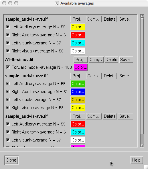
The dialog for managing available averages.
In the example of The dialog for managing available averages., the first item is an average computed within mne_browse_raw , the second one contains data loaded from a file with signal-space projection data available, the third one demonstrates multiple data sets loaded from a file with neither projection nor software gradient compensation available, and the last one is a data set loaded from file with software gradient compensation data present. Note that this is now a scrolled window and some of the loaded data may be below or above the current view area.
The Signal-Space Projection (SSP) is one approach to rejection of external disturbances in software. The section presents some relevant details of this method.
Unlike many other noise-cancellation approaches, SSP does not require additional reference sensors to record the disturbance fields. Instead, SSP relies on the fact that the magnetic field distributions generated by the sources in the brain have spatial distributions sufficiently different from those generated by external noise sources. Furthermore, it is implicitly assumed that the linear space spanned by the significant external noise patters has a low dimension.
Without loss of generality we can always decompose any \(n\)-channel measurement \(b(t)\) into its signal and noise components as
Further, if we know that \(b_n(t)\) is well characterized by a few field patterns \(b_1 \dotso b_m\), we can express the disturbance as
where the columns of \(U\) constitute an orthonormal basis for \(b_1 \dotso b_m\), \(c_n(t)\) is an \(m\)-component column vector, and the error term \(e(t)\) is small and does not exhibit any consistent spatial distributions over time, i.e., \(C_e = E \{e e^T\} = I\). Subsequently, we will call the column space of \(U\) the noise subspace. The basic idea of SSP is that we can actually find a small basis set \(b_1 \dotso b_m\) such that the conditions described above are satisfied. We can now construct the orthogonal complement operator
and apply it to \(b(t)\) yielding
since \(P_{\perp}b_n(t) = P_{\perp}Uc_n(t) \approx 0\). The projection operator \(P_{\perp}\) is called the signal-space projection operator and generally provides considerable rejection of noise, suppressing external disturbances by a factor of 10 or more. The effectiveness of SSP depends on two factors:
If the first requirement is not satisfied, some noise will leak through because \(P_{\perp}b_n(t) \neq 0\). If the any of the brain signal vectors \(b_s(t)\) is close to the noise subspace not only the noise but also the signal will be attenuated by the application of \(P_{\perp}\) and, consequently, there might by little gain in signal-to-noise ratio. An example of the effect of SSP demonstrates the effect of SSP on the Vectorview magnetometer data. After the elimination of a three-dimensional noise subspace, the absolute value of the noise is dampened approximately by a factor of 10 and the covariance matrix becomes diagonally dominant.
Since the signal-space projection modifies the signal vectors originating in the brain, it is necessary to apply the projection to the forward solution in the course of inverse computations. This is accomplished by mne_inverse_operator as described in Inverse-operator decomposition. For more information on SSP, please consult the references listed in Signal-space projections.
In the computation of EEG-based source estimates, the MNE software employs the average-electrode reference, which means that the average over all electrode signals \(v_1 \dotso v_p\) is subtracted from each \(v_j\):
It is easy to see that the above equation actually corresponds to the projection:
where
This section describes how the covariance matrices are computed for raw data and epochs.
If a covariance matrix of a raw data is computed the data are checked for artefacts in 200-sample pieces. Let us collect the accepted \(M\) samples from all channels to the vectors \(s_j,\ j = 1, \dotsc ,M\). The estimate of the covariance matrix is then computed as:
where
is the average of the signals over all times. Note that no attempt is made to correct for low frequency drifts in the data. If the contribution of any frequency band is not desired in the covariance matrix estimate, suitable band-pass filter should be applied.
For actual computations, it is convenient to rewrite the expression for the covariance matrix as
The calculation of the covariance matrix is slightly more complicated in the epoch mode. If the bmin and bmax parameters are specified in the covariance matrix description file (see Covariance definitions), baseline correction is first applied to each epoch.
Let the vectors
be the samples from all channels in the baseline corrected epochs used to calculate the covariance matrix. In the above, \(P_r\) is the number of accepted epochs in category \(r\), \(N_r\) is the number of samples in the epochs of category \(r\), and \(R\) is the number of categories.
If the recommended --keepsamplemean option
is specified in the covariance matrix definition file, the baseline
correction is applied to the epochs but the means at individual
samples are not subtracted. Thus the covariance matrix will be computed
as:
where
If keepsamplemean is not specified, we estimate the covariance matrix as
where
and
which reflects the fact that \(N_r\) means are computed for category \(r\). It is easy to see that the expression for the covariance matrix estimate can be cast into a more convenient form
Subtraction of the means at individual samples is useful if it can be expected that the evoked response from previous stimulus extends to part of baseline period of the next one.
Let us assume that we have computed multiple covariance matrix estimates \(\hat{C_1} \dotso \hat{C_Q}\) with corresponding degrees of freedom \(N_1 \dotso N_Q\). We can combine these matrices together as
where
If a signal space projection was on when a covariance matrix
was calculated, information about the projections applied is included
with the covariance matrix when it is saved. These projection data
are read by mne_inverse_operator and
applied to the forward solution as well as appropriate. Inclusion
of the projections into the covariance matrix limits the possibilities
to use the --bad and --proj options in mne_inverse_operator ,
see Inverse-operator decomposition.
To facilitate interactive analysis of raw data, mne_browse_raw can run mne_analyze as a child process. In this mode, mne_analyze is “remote controlled” by mne_browse_raw and will also send replies to mne_browse_raw to keep the two programs synchronized. A practical application of this communication is to view field or potential maps and cortically-constrained source estimates computed from raw data instantly.
The subordinate mne_analyze is started and stopped from Start mne_analyze and Quit mne_analyze in the Windows menu, respectively. The following settings are communicated between the two processes:
The raw data file
If a new raw data file is opened and a subordinate mne_analyze is active, the name of the raw data file is communicated to mne_analyze and a simplified version of the open dialog appears in mne_analyze allowing selection of an inverse operator or are MEG/MRI coordinate transformation. If a raw data file is already open in mne_browse_raw when mne_analyze is started, the open dialog appears immediately.
Time point
When a new time point is selected in mne_browse_raw the mne_analyze time point selection is updated accordingly. Time point selection in mne_analyze is not transferred to mne_browse_raw .
Scales
The vertical scales are kept synchronized between the two programs. In addition, the settings of the sample time limits are communicated from mne_browse_raw to mne_analyze .
Filter
The filter settings are kept synchronized.