MNE-Python reimplements most of MNE-C’s (the original MNE command line utils) functionality and offers transparent scripting. On top of that it extends MNE-C’s functionality considerably (customize events, compute contrasts, group statistics, time-frequency analysis, EEG-sensor space analyses, etc.) It uses the same files as standard MNE unix commands: no need to convert your files to a new system or database.
- Raw data visualization to visualize recordings, can also use mne_browse_raw for extended functionality (see Browsing raw data with mne_browse_raw)
- Epoching: Define epochs, baseline correction, handle conditions etc.
- Averaging to get Evoked data
- Compute SSP projectors to remove ECG and EOG artifacts
- Compute ICA to remove artifacts or select latent sources.
- Maxwell filtering to remove environmental noise.
- Boundary Element Modeling: single and three-layer BEM model creation and solution computation.
- Forward modeling: BEM computation and mesh creation (see The forward solution)
- Linear inverse solvers (dSPM, sLORETA, MNE, LCMV, DICS)
- Sparse inverse solvers (L1/L2 mixed norm MxNE, Gamma Map, Time-Frequency MxNE)
- Connectivity estimation in sensor and source space
- Visualization of sensor and source space data
- Time-frequency analysis with Morlet wavelets (induced power, intertrial coherence, phase lock value) also in the source space
- Spectrum estimation using multi-taper method
- Mixed Source Models combining cortical and subcortical structures
- Dipole Fitting
- Decoding multivariate pattern analyis of M/EEG topographies
- Compute contrasts between conditions, between sensors, across subjects etc.
- Non-parametric statistics in time, space and frequency (including cluster-level)
- Scripting (batch and parallel computing)
- Brain and head surface segmentation for use with BEM models – use Freesurfer.
Note
This package is based on the FIF file format from Neuromag. It can read and convert CTF, BTI/4D, KIT and various EEG formats to FIF.
See Install Python and MNE-Python.
Note
The expected location for the MNE-sample data is
~/mne_data. If you downloaded data and an example asks
you whether to download it again, make sure
the data reside in the examples directory and you run the script from its
current directory.
From IPython e.g. say:
cd examples/preprocessing
%run plot_find_ecg_artifacts.py
Now, launch ipython (Advanced Python shell) using the QT backend, which is best supported across systems:
$ ipython --matplotlib=qt
First, load the mne package:
Note
In IPython, you can press shift-enter with a given cell selected to execute it and advance to the next cell:
import mne
If you’d like to turn information status messages off:
mne.set_log_level('WARNING')
But it’s generally a good idea to leave them on:
mne.set_log_level('INFO')
You can set the default level by setting the environment variable “MNE_LOGGING_LEVEL”, or by having mne-python write preferences to a file:
mne.set_config('MNE_LOGGING_LEVEL', 'WARNING', set_env=True)
Note that the location of the mne-python preferences file (for easier manual editing) can be found using:
By default logging messages print to the console, but look at
mne.set_log_file() to save output to a file.
from mne.datasets import sample  # noqa
data_path = sample.data_path()
raw_fname = data_path + '/MEG/sample/sample_audvis_filt-0-40_raw.fif'
print(raw_fname)
Out:
/home/ubuntu/mne_data/MNE-sample-data/MEG/sample/sample_audvis_filt-0-40_raw.fif
Note
The MNE sample dataset should be downloaded automatically but be patient (approx. 2GB)
Read data from file:
raw = mne.io.read_raw_fif(raw_fname)
print(raw)
print(raw.info)
Out:
Opening raw data file /home/ubuntu/mne_data/MNE-sample-data/MEG/sample/sample_audvis_filt-0-40_raw.fif...
    Read a total of 4 projection items:
        PCA-v1 (1 x 10²)  idle
        PCA-v2 (1 x 10²)  idle
        PCA-v3 (1 x 10²)  idle
        Average EEG reference (1 x 60)  idle
    Range : 6450 ... 48149 =     42.956 ...   320.665 secs
Ready.
Current compensation grade : 0
<Raw  |  sample_audvis_filt-0-40_raw.fif, n_channels x n_times : 376 x 41700 (277.7 sec), ~3.7 MB, data not loaded>
<Info | 19 non-empty fields
    bads : list | MEG 2443, EEG 053
    buffer_size_sec : numpy.float64 | 13.3196808772
    ch_names : list | MEG 0113, MEG 0112, MEG 0111, MEG 0122, MEG 0123, ...
    chs : list | 376 items (EOG: 1, EEG: 60, STIM: 9, GRAD: 204, MAG: 102)
    comps : list | 0 items
    custom_ref_applied : bool | False
    dev_head_t : 'mne.transforms.Transform | 3 items
    dig : list | 146 items
    events : list | 0 items
    file_id : dict | 4 items
    highpass : float | 0.10000000149 Hz
    hpi_meas : list | 1 items
    hpi_results : list | 1 items
    lowpass : float | 40.0 Hz
    meas_date : numpy.ndarray | 2002-12-03 19:01:10
    meas_id : dict | 4 items
    nchan : int | 376
    projs : list | PCA-v1: off, PCA-v2: off, PCA-v3: off, ...
    sfreq : float | 150.153747559 Hz
    acq_pars : NoneType
    acq_stim : NoneType
    ctf_head_t : NoneType
    description : NoneType
    dev_ctf_t : NoneType
    experimenter : NoneType
    hpi_subsystem : NoneType
    kit_system_id : NoneType
    line_freq : NoneType
    proj_id : NoneType
    proj_name : NoneType
    subject_info : NoneType
    xplotter_layout : NoneType
>
Look at the channels in raw:
print(raw.ch_names)
Out:
[u'MEG 0113', u'MEG 0112', u'MEG 0111', u'MEG 0122', u'MEG 0123', u'MEG 0121', u'MEG 0132', u'MEG 0133', u'MEG 0131', u'MEG 0143', u'MEG 0142', u'MEG 0141', u'MEG 0213', u'MEG 0212', u'MEG 0211', u'MEG 0222', u'MEG 0223', u'MEG 0221', u'MEG 0232', u'MEG 0233', u'MEG 0231', u'MEG 0243', u'MEG 0242', u'MEG 0241', u'MEG 0313', u'MEG 0312', u'MEG 0311', u'MEG 0322', u'MEG 0323', u'MEG 0321', u'MEG 0333', u'MEG 0332', u'MEG 0331', u'MEG 0343', u'MEG 0342', u'MEG 0341', u'MEG 0413', u'MEG 0412', u'MEG 0411', u'MEG 0422', u'MEG 0423', u'MEG 0421', u'MEG 0432', u'MEG 0433', u'MEG 0431', u'MEG 0443', u'MEG 0442', u'MEG 0441', u'MEG 0513', u'MEG 0512', u'MEG 0511', u'MEG 0523', u'MEG 0522', u'MEG 0521', u'MEG 0532', u'MEG 0533', u'MEG 0531', u'MEG 0542', u'MEG 0543', u'MEG 0541', u'MEG 0613', u'MEG 0612', u'MEG 0611', u'MEG 0622', u'MEG 0623', u'MEG 0621', u'MEG 0633', u'MEG 0632', u'MEG 0631', u'MEG 0642', u'MEG 0643', u'MEG 0641', u'MEG 0713', u'MEG 0712', u'MEG 0711', u'MEG 0723', u'MEG 0722', u'MEG 0721', u'MEG 0733', u'MEG 0732', u'MEG 0731', u'MEG 0743', u'MEG 0742', u'MEG 0741', u'MEG 0813', u'MEG 0812', u'MEG 0811', u'MEG 0822', u'MEG 0823', u'MEG 0821', u'MEG 0913', u'MEG 0912', u'MEG 0911', u'MEG 0923', u'MEG 0922', u'MEG 0921', u'MEG 0932', u'MEG 0933', u'MEG 0931', u'MEG 0942', u'MEG 0943', u'MEG 0941', u'MEG 1013', u'MEG 1012', u'MEG 1011', u'MEG 1023', u'MEG 1022', u'MEG 1021', u'MEG 1032', u'MEG 1033', u'MEG 1031', u'MEG 1043', u'MEG 1042', u'MEG 1041', u'MEG 1112', u'MEG 1113', u'MEG 1111', u'MEG 1123', u'MEG 1122', u'MEG 1121', u'MEG 1133', u'MEG 1132', u'MEG 1131', u'MEG 1142', u'MEG 1143', u'MEG 1141', u'MEG 1213', u'MEG 1212', u'MEG 1211', u'MEG 1223', u'MEG 1222', u'MEG 1221', u'MEG 1232', u'MEG 1233', u'MEG 1231', u'MEG 1243', u'MEG 1242', u'MEG 1241', u'MEG 1312', u'MEG 1313', u'MEG 1311', u'MEG 1323', u'MEG 1322', u'MEG 1321', u'MEG 1333', u'MEG 1332', u'MEG 1331', u'MEG 1342', u'MEG 1343', u'MEG 1341', u'MEG 1412', u'MEG 1413', u'MEG 1411', u'MEG 1423', u'MEG 1422', u'MEG 1421', u'MEG 1433', u'MEG 1432', u'MEG 1431', u'MEG 1442', u'MEG 1443', u'MEG 1441', u'MEG 1512', u'MEG 1513', u'MEG 1511', u'MEG 1522', u'MEG 1523', u'MEG 1521', u'MEG 1533', u'MEG 1532', u'MEG 1531', u'MEG 1543', u'MEG 1542', u'MEG 1541', u'MEG 1613', u'MEG 1612', u'MEG 1611', u'MEG 1622', u'MEG 1623', u'MEG 1621', u'MEG 1632', u'MEG 1633', u'MEG 1631', u'MEG 1643', u'MEG 1642', u'MEG 1641', u'MEG 1713', u'MEG 1712', u'MEG 1711', u'MEG 1722', u'MEG 1723', u'MEG 1721', u'MEG 1732', u'MEG 1733', u'MEG 1731', u'MEG 1743', u'MEG 1742', u'MEG 1741', u'MEG 1813', u'MEG 1812', u'MEG 1811', u'MEG 1822', u'MEG 1823', u'MEG 1821', u'MEG 1832', u'MEG 1833', u'MEG 1831', u'MEG 1843', u'MEG 1842', u'MEG 1841', u'MEG 1912', u'MEG 1913', u'MEG 1911', u'MEG 1923', u'MEG 1922', u'MEG 1921', u'MEG 1932', u'MEG 1933', u'MEG 1931', u'MEG 1943', u'MEG 1942', u'MEG 1941', u'MEG 2013', u'MEG 2012', u'MEG 2011', u'MEG 2023', u'MEG 2022', u'MEG 2021', u'MEG 2032', u'MEG 2033', u'MEG 2031', u'MEG 2042', u'MEG 2043', u'MEG 2041', u'MEG 2113', u'MEG 2112', u'MEG 2111', u'MEG 2122', u'MEG 2123', u'MEG 2121', u'MEG 2133', u'MEG 2132', u'MEG 2131', u'MEG 2143', u'MEG 2142', u'MEG 2141', u'MEG 2212', u'MEG 2213', u'MEG 2211', u'MEG 2223', u'MEG 2222', u'MEG 2221', u'MEG 2233', u'MEG 2232', u'MEG 2231', u'MEG 2242', u'MEG 2243', u'MEG 2241', u'MEG 2312', u'MEG 2313', u'MEG 2311', u'MEG 2323', u'MEG 2322', u'MEG 2321', u'MEG 2332', u'MEG 2333', u'MEG 2331', u'MEG 2343', u'MEG 2342', u'MEG 2341', u'MEG 2412', u'MEG 2413', u'MEG 2411', u'MEG 2423', u'MEG 2422', u'MEG 2421', u'MEG 2433', u'MEG 2432', u'MEG 2431', u'MEG 2442', u'MEG 2443', u'MEG 2441', u'MEG 2512', u'MEG 2513', u'MEG 2511', u'MEG 2522', u'MEG 2523', u'MEG 2521', u'MEG 2533', u'MEG 2532', u'MEG 2531', u'MEG 2543', u'MEG 2542', u'MEG 2541', u'MEG 2612', u'MEG 2613', u'MEG 2611', u'MEG 2623', u'MEG 2622', u'MEG 2621', u'MEG 2633', u'MEG 2632', u'MEG 2631', u'MEG 2642', u'MEG 2643', u'MEG 2641', u'STI 001', u'STI 002', u'STI 003', u'STI 004', u'STI 005', u'STI 006', u'STI 014', u'STI 015', u'STI 016', u'EEG 001', u'EEG 002', u'EEG 003', u'EEG 004', u'EEG 005', u'EEG 006', u'EEG 007', u'EEG 008', u'EEG 009', u'EEG 010', u'EEG 011', u'EEG 012', u'EEG 013', u'EEG 014', u'EEG 015', u'EEG 016', u'EEG 017', u'EEG 018', u'EEG 019', u'EEG 020', u'EEG 021', u'EEG 022', u'EEG 023', u'EEG 024', u'EEG 025', u'EEG 026', u'EEG 027', u'EEG 028', u'EEG 029', u'EEG 030', u'EEG 031', u'EEG 032', u'EEG 033', u'EEG 034', u'EEG 035', u'EEG 036', u'EEG 037', u'EEG 038', u'EEG 039', u'EEG 040', u'EEG 041', u'EEG 042', u'EEG 043', u'EEG 044', u'EEG 045', u'EEG 046', u'EEG 047', u'EEG 048', u'EEG 049', u'EEG 050', u'EEG 051', u'EEG 052', u'EEG 053', u'EEG 054', u'EEG 055', u'EEG 056', u'EEG 057', u'EEG 058', u'EEG 059', u'EEG 060', u'EOG 061']
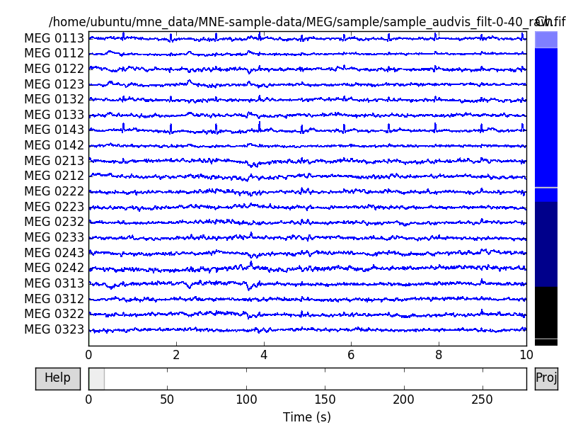
Read and plot a segment of raw data
start, stop = raw.time_as_index([100, 115])  # 100 s to 115 s data segment
data, times = raw[:, start:stop]
print(data.shape)
print(times.shape)
data, times = raw[2:20:3, start:stop]  # access underlying data
raw.plot()
Out:
(376, 2252)
(2252,)
Save a segment of 150s of raw data (MEG only):
picks = mne.pick_types(raw.info, meg=True, eeg=False, stim=True,
                       exclude='bads')
raw.save('sample_audvis_meg_raw.fif', tmin=0, tmax=150, picks=picks,
         overwrite=True)
Out:
Writing /home/ubuntu/mne-python/tutorials/sample_audvis_meg_raw.fif
Closing /home/ubuntu/mne-python/tutorials/sample_audvis_meg_raw.fif [done]
First extract events:
events = mne.find_events(raw, stim_channel='STI 014')
print(events[:5])
Out:
319 events found
Events id: [ 1  2  3  4  5 32]
[[6994    0    2]
 [7086    0    3]
 [7192    0    1]
 [7304    0    4]
 [7413    0    2]]
Note that, by default, we use stim_channel=’STI 014’. If you have a different system (e.g., a newer system that uses channel ‘STI101’ by default), you can use the following to set the default stim channel to use for finding events:
mne.set_config('MNE_STIM_CHANNEL', 'STI101', set_env=True)
Events are stored as a 2D numpy array where the first column is the time instant and the last one is the event number. It is therefore easy to manipulate.
Define epochs parameters:
event_id = dict(aud_l=1, aud_r=2)  # event trigger and conditions
tmin = -0.2  # start of each epoch (200ms before the trigger)
tmax = 0.5  # end of each epoch (500ms after the trigger)
Exclude some channels (original bads + 2 more):
raw.info['bads'] += ['MEG 2443', 'EEG 053']
The variable raw.info[‘bads’] is just a python list.
Pick the good channels, excluding raw.info[‘bads’]:
picks = mne.pick_types(raw.info, meg=True, eeg=True, eog=True, stim=False,
                       exclude='bads')
Alternatively one can restrict to magnetometers or gradiometers with:
mag_picks = mne.pick_types(raw.info, meg='mag', eog=True, exclude='bads')
grad_picks = mne.pick_types(raw.info, meg='grad', eog=True, exclude='bads')
Define the baseline period:
baseline = (None, 0) # means from the first instant to t = 0
Define peak-to-peak rejection parameters for gradiometers, magnetometers and EOG:
reject = dict(grad=4000e-13, mag=4e-12, eog=150e-6)
Read epochs:
epochs = mne.Epochs(raw, events, event_id, tmin, tmax, proj=True, picks=picks,
                    baseline=baseline, preload=False, reject=reject)
print(epochs)
Out:
145 matching events found
Created an SSP operator (subspace dimension = 4)
4 projection items activated
<Epochs  |  n_events : 145 (good & bad), tmin : -0.199795213158 (s), tmax : 0.499488032896 (s), baseline : (None, 0), ~3.7 MB, data not loaded,
 'aud_l': 72, 'aud_r': 73>
Get single epochs for one condition:
epochs_data = epochs['aud_l'].get_data()
print(epochs_data.shape)
Out:
Loading data for 72 events and 106 original time points ...
    Rejecting  epoch based on EOG : [u'EOG 061']
    Rejecting  epoch based on EOG : [u'EOG 061']
    Rejecting  epoch based on EOG : [u'EOG 061']
    Rejecting  epoch based on EOG : [u'EOG 061']
    Rejecting  epoch based on EOG : [u'EOG 061']
    Rejecting  epoch based on MAG : [u'MEG 1711']
    Rejecting  epoch based on EOG : [u'EOG 061']
    Rejecting  epoch based on EOG : [u'EOG 061']
    Rejecting  epoch based on EOG : [u'EOG 061']
    Rejecting  epoch based on EOG : [u'EOG 061']
    Rejecting  epoch based on EOG : [u'EOG 061']
    Rejecting  epoch based on EOG : [u'EOG 061']
    Rejecting  epoch based on EOG : [u'EOG 061']
    Rejecting  epoch based on EOG : [u'EOG 061']
    Rejecting  epoch based on EOG : [u'EOG 061']
    Rejecting  epoch based on EOG : [u'EOG 061']
    Rejecting  epoch based on EOG : [u'EOG 061']
17 bad epochs dropped
(55, 365, 106)
epochs_data is a 3D array of dimension (55 epochs, 365 channels, 106 time instants).
Scipy supports read and write of matlab files. You can save your single trials with:
from scipy import io  # noqa
io.savemat('epochs_data.mat', dict(epochs_data=epochs_data), oned_as='row')
or if you want to keep all the information about the data you can save your epochs in a fif file:
epochs.save('sample-epo.fif')
Out:
Loading data for 145 events and 106 original time points ...
    Rejecting  epoch based on EOG : [u'EOG 061']
    Rejecting  epoch based on EOG : [u'EOG 061']
    Rejecting  epoch based on EOG : [u'EOG 061']
    Rejecting  epoch based on EOG : [u'EOG 061']
    Rejecting  epoch based on EOG : [u'EOG 061']
    Rejecting  epoch based on EOG : [u'EOG 061']
    Rejecting  epoch based on EOG : [u'EOG 061']
    Rejecting  epoch based on EOG : [u'EOG 061']
    Rejecting  epoch based on MAG : [u'MEG 1711']
    Rejecting  epoch based on EOG : [u'EOG 061']
    Rejecting  epoch based on EOG : [u'EOG 061']
    Rejecting  epoch based on EOG : [u'EOG 061']
    Rejecting  epoch based on MAG : [u'MEG 1711']
    Rejecting  epoch based on EOG : [u'EOG 061']
    Rejecting  epoch based on EOG : [u'EOG 061']
    Rejecting  epoch based on EOG : [u'EOG 061']
    Rejecting  epoch based on EOG : [u'EOG 061']
    Rejecting  epoch based on EOG : [u'EOG 061']
    Rejecting  epoch based on EOG : [u'EOG 061']
    Rejecting  epoch based on EOG : [u'EOG 061']
    Rejecting  epoch based on EOG : [u'EOG 061']
    Rejecting  epoch based on EOG : [u'EOG 061']
    Rejecting  epoch based on EOG : [u'EOG 061']
    Rejecting  epoch based on EOG : [u'EOG 061']
    Rejecting  epoch based on EOG : [u'EOG 061']
    Rejecting  epoch based on EOG : [u'EOG 061']
    Rejecting  epoch based on EOG : [u'EOG 061']
    Rejecting  epoch based on EOG : [u'EOG 061']
    Rejecting  epoch based on EOG : [u'EOG 061']
29 bad epochs dropped
Loading data for 1 events and 106 original time points ...
Loading data for 116 events and 106 original time points ...
and read them later with:
saved_epochs = mne.read_epochs('sample-epo.fif')
Out:
Reading sample-epo.fif ...
    Read a total of 4 projection items:
        PCA-v1 (1 x 10²) active
        PCA-v2 (1 x 10²) active
        PCA-v3 (1 x 10²) active
        Average EEG reference (1 x 60) active
    Found the data of interest:
        t =    -199.80 ...     499.49 ms (None)
        0 CTF compensation matrices available
116 matching events found
Created an SSP operator (subspace dimension = 4)
116 matching events found
Created an SSP operator (subspace dimension = 4)
4 projection items activated
Compute evoked responses for auditory responses by averaging and plot it:
evoked = epochs['aud_l'].average()
print(evoked)
evoked.plot()
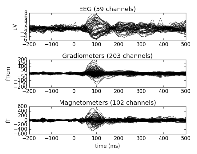
Out:
<Evoked | comment : 'aud_l', kind : average, time : [-0.199795, 0.499488], n_epochs : 55, n_channels x n_times : 364 x 106, ~4.0 MB>
Exercise
max_in_each_epoch = [e.max() for e in epochs['aud_l']]  # doctest:+ELLIPSIS
print(max_in_each_epoch[:4])  # doctest:+ELLIPSIS
Out:
[1.9375167201631345e-05, 1.640551698642913e-05, 1.8545377810380145e-05, 2.0412807568093327e-05]
It is also possible to read evoked data stored in a fif file:
evoked_fname = data_path + '/MEG/sample/sample_audvis-ave.fif'
evoked1 = mne.read_evokeds(
    evoked_fname, condition='Left Auditory', baseline=(None, 0), proj=True)
Out:
Reading /home/ubuntu/mne_data/MNE-sample-data/MEG/sample/sample_audvis-ave.fif ...
    Read a total of 4 projection items:
        PCA-v1 (1 x 10²) active
        PCA-v2 (1 x 10²) active
        PCA-v3 (1 x 10²) active
        Average EEG reference (1 x 60) active
    Found the data of interest:
        t =    -199.80 ...     499.49 ms (Left Auditory)
        0 CTF compensation matrices available
        nave = 55 - aspect type = 100
Projections have already been applied. Setting proj attribute to True.
Applying baseline correction (mode: mean)
Or another one stored in the same file:
evoked2 = mne.read_evokeds(
    evoked_fname, condition='Right Auditory', baseline=(None, 0), proj=True)
Out:
Reading /home/ubuntu/mne_data/MNE-sample-data/MEG/sample/sample_audvis-ave.fif ...
    Read a total of 4 projection items:
        PCA-v1 (1 x 10²) active
        PCA-v2 (1 x 10²) active
        PCA-v3 (1 x 10²) active
        Average EEG reference (1 x 60) active
    Found the data of interest:
        t =    -199.80 ...     499.49 ms (Right Auditory)
        0 CTF compensation matrices available
        nave = 61 - aspect type = 100
Projections have already been applied. Setting proj attribute to True.
Applying baseline correction (mode: mean)
Two evoked objects can be contrasted using mne.combine_evoked().
This function can use weights='equal', which provides a simple
element-by-element subtraction (and sets the
mne.Evoked.nave attribute properly based on the underlying number
of trials) using either equivalent call:
contrast = mne.combine_evoked([evoked1, evoked2], weights=[0.5, -0.5])
contrast = mne.combine_evoked([evoked1, -evoked2], weights='equal')
print(contrast)
Out:
<Evoked | comment : '0.500 * Left Auditory + 0.500 * -Right Auditory', kind : average, time : [-0.199795, 0.499488], n_epochs : 116, n_channels x n_times : 376 x 421, ~4.9 MB>
To do a weighted sum based on the number of averages, which will give
you what you would have gotten from pooling all trials together in
mne.Epochs before creating the mne.Evoked instance,
you can use weights='nave':
average = mne.combine_evoked([evoked1, evoked2], weights='nave')
print(contrast)
Out:
<Evoked | comment : '0.500 * Left Auditory + 0.500 * -Right Auditory', kind : average, time : [-0.199795, 0.499488], n_epochs : 116, n_channels x n_times : 376 x 421, ~4.9 MB>
Instead of dealing with mismatches in the number of averages, we can use
trial-count equalization before computing a contrast, which can have some
benefits in inverse imaging (note that here weights='nave' will
give the same result as weights='equal'):
epochs_eq = epochs.copy().equalize_event_counts(['aud_l', 'aud_r'])[0]
evoked1, evoked2 = epochs_eq['aud_l'].average(), epochs_eq['aud_r'].average()
print(evoked1)
print(evoked2)
contrast = mne.combine_evoked([evoked1, -evoked2], weights='equal')
print(contrast)
Out:
Dropped 6 epochs
<Evoked  |  comment : 'aud_l', kind : average, time : [-0.199795, 0.499488], n_epochs : 55, n_channels x n_times : 364 x 106, ~4.0 MB>
<Evoked  |  comment : 'aud_r', kind : average, time : [-0.199795, 0.499488], n_epochs : 55, n_channels x n_times : 364 x 106, ~4.0 MB>
<Evoked  |  comment : '0.500 * aud_l + 0.500 * -aud_r', kind : average, time : [-0.199795, 0.499488], n_epochs : 110, n_channels x n_times : 364 x 106, ~4.0 MB>
Define parameters:
import numpy as np  # noqa
n_cycles = 2  # number of cycles in Morlet wavelet
freqs = np.arange(7, 30, 3)  # frequencies of interest
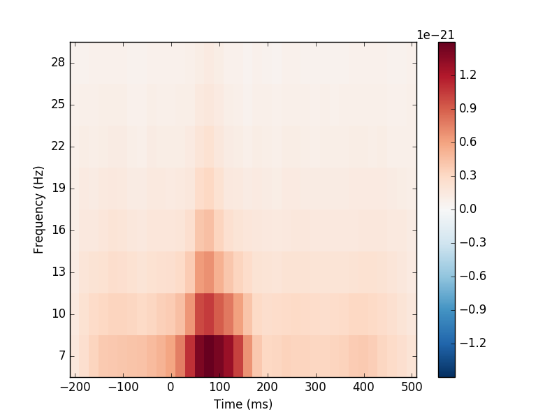
Compute induced power and phase-locking values and plot gradiometers:
from mne.time_frequency import tfr_morlet  # noqa
power, itc = tfr_morlet(epochs, freqs=freqs, n_cycles=n_cycles,
                        return_itc=True, decim=3, n_jobs=1)
power.plot([power.ch_names.index('MEG 1332')])
Out:
Loading data for 116 events and 106 original time points ...
No baseline correction applied
Import the required functions:
from mne.minimum_norm import apply_inverse, read_inverse_operator # noqa
Read the inverse operator:
fname_inv = data_path + '/MEG/sample/sample_audvis-meg-oct-6-meg-inv.fif'
inverse_operator = read_inverse_operator(fname_inv)
Out:
Reading inverse operator decomposition from /home/ubuntu/mne_data/MNE-sample-data/MEG/sample/sample_audvis-meg-oct-6-meg-inv.fif...
    Reading inverse operator info...
    [done]
    Reading inverse operator decomposition...
    [done]
    305 x 305 full covariance (kind = 1) found.
    Read a total of 4 projection items:
        PCA-v1 (1 x 10²) active
        PCA-v2 (1 x 10²) active
        PCA-v3 (1 x 10²) active
        Average EEG reference (1 x 60) active
    Noise covariance matrix read.
    22494 x 22494 diagonal covariance (kind = 2) found.
    Source covariance matrix read.
    22494 x 22494 diagonal covariance (kind = 6) found.
    Orientation priors read.
    22494 x 22494 diagonal covariance (kind = 5) found.
    Depth priors read.
    Did not find the desired covariance matrix (kind = 3)
    Reading a source space...
    Computing patch statistics...
    Patch information added...
    Distance information added...
    [done]
    Reading a source space...
    Computing patch statistics...
    Patch information added...
    Distance information added...
    [done]
    2 source spaces read
    Read a total of 4 projection items:
        PCA-v1 (1 x 10²) active
        PCA-v2 (1 x 10²) active
        PCA-v3 (1 x 10²) active
        Average EEG reference (1 x 60) active
    Source spaces transformed to the inverse solution coordinate frame
Define the inverse parameters:
snr = 3.0
lambda2 = 1.0 / snr ** 2
method = "dSPM"
Compute the inverse solution:
stc = apply_inverse(evoked, inverse_operator, lambda2, method)
Out:
Preparing the inverse operator for use...
    Scaled noise and source covariance from nave = 1 to nave = 55
    Created the regularized inverter
    Created an SSP operator (subspace dimension = 3)
    Created the whitener using a full noise covariance matrix (3 small eigenvalues omitted)
    Computing noise-normalization factors (dSPM)...
[done]
Picked 305 channels from the data
Computing inverse...
(eigenleads need to be weighted)...
combining the current components...
(dSPM)...
[done]
Save the source time courses to disk:
stc.save('mne_dSPM_inverse')
Out:
Writing STC to disk...
[done]
Now, let’s compute dSPM on a raw file within a label:
fname_label = data_path + '/MEG/sample/labels/Aud-lh.label'
label = mne.read_label(fname_label)
Compute inverse solution during the first 15s:
from mne.minimum_norm import apply_inverse_raw  # noqa
start, stop = raw.time_as_index([0, 15])  # read the first 15s of data
stc = apply_inverse_raw(raw, inverse_operator, lambda2, method, label,
                        start, stop)
Out:
Preparing the inverse operator for use...
    Scaled noise and source covariance from nave = 1 to nave = 1
    Created the regularized inverter
    Created an SSP operator (subspace dimension = 3)
    Created the whitener using a full noise covariance matrix (3 small eigenvalues omitted)
    Computing noise-normalization factors (dSPM)...
[done]
Picked 305 channels from the data
Computing inverse...
(eigenleads need to be weighted)...
combining the current components...
[done]
Save result in stc files:
stc.save('mne_dSPM_raw_inverse_Aud')
Out:
Writing STC to disk...
[done]
- detect heart beat QRS component
- detect eye blinks and EOG artifacts
- compute SSP projections to remove ECG or EOG artifacts
- compute Independent Component Analysis (ICA) to remove artifacts or select latent sources
- estimate noise covariance matrix from Raw and Epochs
- visualize cross-trial response dynamics using epochs images
- compute forward solutions
- estimate power in the source space
- estimate connectivity in sensor and source space
- morph stc from one brain to another for group studies
- compute mass univariate statistics base on custom contrasts
- visualize source estimates
- export raw, epochs, and evoked data to other python data analysis libraries e.g. pandas
- and many more things …
Browse the examples gallery.
print("Done!")
Out:
Done!
Total running time of the script: ( 0 minutes 14.790 seconds)