![]()
Contents
Interactive analysis of the MEG/EEG data and source estimates is facilitated by the mne_analyze tool. Its features include:
See mne_analyze for command line options.
Note
Before starting mne_analyze the SUBJECTS_DIR environment variable has to be set.
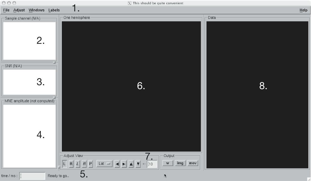
The main window of mne_analyze.
The main window of mne_analyze shown in The main window of mne_analyze. has the following components:
The File shown in The file menu contains the following items:
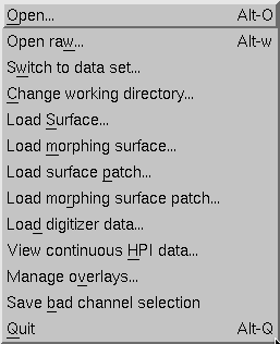
The file menu
Open…
Load a new data set and an inverse operator. For details, see Loading data.
Open raw…
Load epoch data from a raw data file. For details, see Loading epochs from a raw data file.
Switch to data set…
If multiple data sets or epochs from a raw data file are loaded, this menu item brings up a list to switch between the data sets or epochs.
Change working directory…
Change the working directory of this program. This will usually be the directory where your MEG/EEG data and inverse operator are located.
Load surface…
Load surface reconstructions for the subject whose data you are analyzing, see The surface display.
Load morphing surface…
Load surface reconstructions of another subject for morphing, see Morphing.
Load surface patch…
Load a curved or flattened surface patch, see The surface display.
Load morphing surface patch…
Load a curved or flattened surface patch for morphing, see Morphing.
Load digitizer data…
Load digitizer data for coordinate frame alignment, see Coordinate frame alignment.
View continuous HPI data…
Load a data file containing continuous head position information, see Viewing continuous HPI data.
Manage overlays…
Bring up the overlay manager to import data from stc and w files, see Overlays.
Save bad channel selection
Save the current bad channel selection created in the topographical data display, see Data displays.
Quit
Quit the program.
The contents of the Adjust menu is shown in The Adjust menu.:
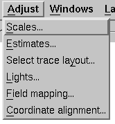
The Adjust menu.
Scales
Adjust the scales of the data display.
Estimates…
Adjust the properties of the displayed current estimates, see Working with current estimates.
Select trace layout…
Select the layout for the topographical display, see Data displays.
Lights…
Adjust the lighting of the scenes in the main display and the viewer, see Working with current estimates and The viewer.
Field mapping…
Adjust the field mapping preferences, see Magnetic field and electric potential maps.
Coordinate alignment…
Establish a coordinate transformation between the MEG and MRI coordinate frames, see Coordinate frame alignment.
The contents of the file menu is shown in The View menu.:
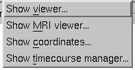
The View menu.
Show viewer…
Loads additional surfaces and pops up the viewer window. The functions available in the viewer are discussed in The viewer.
Show MRI viewer…
Bring up the tkmedit program to view MRI slices, see Working with the MRI viewer.
Show coordinates…
Show the coordinates of a vertex, see Selecting vertices.
Show timecourse manager…
Brings up the timecourse manager if some timecourses are available. Timecourses are discussed in Inquiring timecourses.
The contents of the Labels menu is shown in The Labels menu.. ROI analysis with help of labels is discussed in detail in Inquiring timecourses.
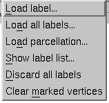
The Labels menu.
The label menu contains the following items:
Load label…
Loads one label file for ROI analysis.
Load all labels…
Loads all label files available in a directory for ROI analysis.
Load parcellation…
Load cortical parcellation data produced by FreeSurfer from directory $SUBJECTS_DIR/$SUBJECT/label and add the cortical regions defined to the label list.
Show label list…
Shows a list of all currently loaded labels for ROI analysis.
Discard all labels
Discard all labels loaded so far. The label list window will be hidden.
Clear marked vertices
Clear the label outline or a label created interactively.
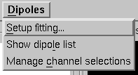
The contents of the dipoles menu is shown in The dipole fitting menu.:
The dipole fitting menu.
Setup fitting…
Define the dipole fitting parameters, see Dipole fitting parameters.
Show dipole list…
Show the list of imported and fitted dipoles, see The dipole list.
Manage channel selections…
Manage the selections of channels used in dipole fitting, see Channel selections.
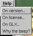
The contents of the Help menu is shown in The Help menu.:
The Help menu.
On version…
Displays the version and compilation date of the program.
On license…
Displays the license information.
On GLX…
Displays information about the OpenGL rendering context. If you experience poor graphics performance, check that the window that pops up from here says that you have a Direct rendering context . If not, either your graphics card or driver software needs an update.
Why the beep?
In some simple error situations, mne_analyze does not popup an error dialog but refuses the action and rings the bell. The reason for this can be displayed through this help menu item.
When you select Open… from the File menu the data loading dialog shown in The open dialog. appears. It has four sections:
inv .mri/T1-neuromag/sets under the subject’s
FreeSurfer directory. The Default button
uses the default transformation file which must be called $SUBJECTS_DIR/$SUBJECT/bem/$SUBJECT-trans.fif .
This can be one of the MRI description files in mri/T1-neuromag/sets or
a transformation file stored from mne_analyze ,
see Coordinate frame alignment.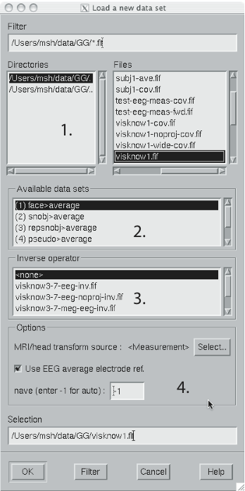
The open dialog.
After the data set(s) has been selected, the following actions will take place:
If multiple data sets are loaded each data set has the following individual settings:
If a data set has not been previously displayed, the currently active settings are copied to the data set.
Note
If you double click on an inverse operator file name displayed in the Inverse operator list, the command used to produced this file will be displayed in a message dialog.
Instead of an evoked-response data file it is possible to load epochs of data (single trials) from a raw data file. This option is invoked from File/Open raw… . The file selection box is identical to the one used for evoked responses (The open dialog.) except that data set selector is replaced by the epoch selector show in The raw data epoch selector..
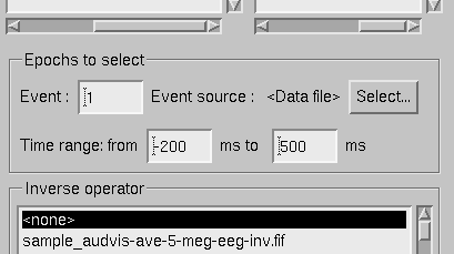
The raw data epoch selector.
The epoch selector contains the following controls:
Once the settings have been accepted by clicking OK , the first matching epoch will be displayed. You can switch between epochs using the data set list accessible through Switch to data set… in the File menu.
The MEG and EEG signals can be viewed in two ways:
In both the sample channel display and the topographical display, current time point can be selected with a left mouse click. In addition, time point of interest can be entered numerically in the text box at the bottom left corner of the main display.
A selection of channels is always shown in the right most part of the main display. The topographical layout to use is selected from Adjust/Select trace layout… , which brings up a window with a list of available layouts. The system-wide layouts reside in $MNE_ROOT/share/mne_analyze/lout. In addition any layout files residing in $HOME/.mne/lout are listed. The format of the layout files and selection of the default layout is discussed in Full view layout.
Several actions can be performed with the mouse in the topographical data display:
Left button click
Selects a time point of interest.
Left button click with control key
Selects a time point of interest and selects the channel under the pointer to the sample channel display.
Left button drag with shift key
Enlarges the view to contain only channels in the selected area.
Middle button click or drag
Marks this channel as bad and clears all previously marked bad channel. This action is only available if an inverse operator is not loaded. An inverse operator dictates the selection of bad channels. The current bad channel selection can be applied to the data from File/Save bad channel selection .
Middle button click or drag with control key
Extends the bad channel selection without clearing the previously active bad channels.
Right button
Adjusts the channel selection used for dipole fitting in the same way as the middle button selects bad channels. For more information on channel selections, see Channel selections.
The sample channel display shows one of the measurement channels at the upper left corner of the mne_analyze user interface. A time point can be selected with a left mouse click. In addition, the following keyboard functions are associated with the sample channel display:
Down
Change the sample channel to the next channel in the scanning order.
Up
Change the sample channel to the previous channel in the scanning order.
Right
Move forward in time by 1 ms.
Control Right
Move forward in time by 5 ms.
Left
Move backward in time by 1 ms.
Control Left
Move backward in time by 5 ms.
The scales of the topographical and sample channel display can be adjusted from the Scales dialog which is invoked by selecting Adjust/Scales… from the menus. The Scales dialog shown in The Scales dialog. has the following entries:
Analyze range min [ms]
Specifies the lower limit of the time range of data to be shown.
Analyze range max [ms]
Specifies the upper limit of the time range of data to be shown.
Use full time range
If this box is checked, all data available in the data file will be shown.
Baseline min [ms]
Specifies the lower time limit of the baseline.
Baseline max [ms]
Specifies the upper time limit of the baseline.
Baseline in use
Baseline subtraction can be switched on and off from this button.
MEG amp min [fT/cm]
Lower limit of the vertical scale of planar gradiometer MEG channels.
MEG amp max [fT/cm]
Upper limit of the vertical scale of planar gradiometer MEG channels.
MEG axmult [cm]
The vertical scale of MEG magnetometers and axial gradiometers will be obtained by multiplying the planar gradiometer vertical scale limits by this value, given in centimeters.
EEG amp min [muV]
Lower limit of the vertical scale of EEG channels.
EEG amp max [muV]
Upper limit of the vertical scale of EEG channels.
Show stimulus channel
Show the digital trigger channel data in the sample view together with the sample channel.
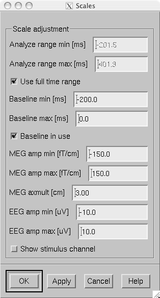
The Scales dialog.
In mne_analyze , the current estimates are visualized on inflated or folded cortical surfaces. There are two visualization displays: the surface display, which is always visible, and the 3D viewer which is invoked from the Windows/Show viewer… menu selection, see The viewer.
A total of eight surfaces or patches can be assigned to the surface display:
When File/Load surface… or File/Load morphing surface… is invoked, the surface selection dialog shown in The surface selection dialog. appears.
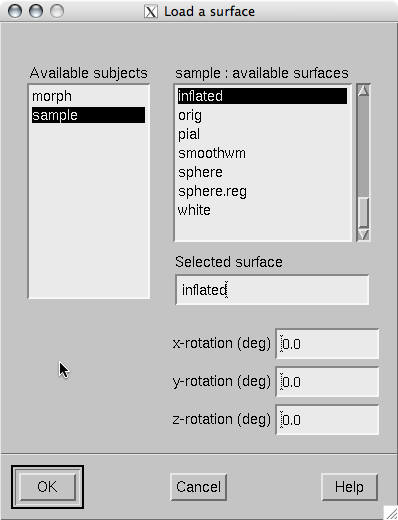
The surface selection dialog.
The dialog has the following components:
List of subjects
This list contains the subjects available in the directory set with theSUBJECTS_DIRenvironment variable.
List of available surfaces for the selected subject
Lists the surfaces available for the current subject. When you click on an item in this list, it appears in the Selected surface text field.
x-rotation (deg)
Specifies the initial rotation of the surface around the x (left to right) axis. Positive angle means a counterclockwise rotation when the surface is looked at from the direction of the positive x axis. Sometimes a more pleasing visualization is obtained when this rotations are specified when the surface is loaded.
y-rotation (deg)
Specifies the initial rotation of the surface around the y (back to front) axis.
z-rotation (deg)
Specifies the initial rotation of the surface around the z (bottom to up) axis.
The surface patches are loaded with help of the patch selection dialog, which appears when File/Load surface patch… or File/Load morphing surface patch… is selected. This dialog, shown in The patch selection dialog., contains a list of available patches and the possibility to rotate the a flat patch counterclockwise by the specified number of degrees from its original orientation. The patch is automatically associated with the correct hemisphere on the basis of the two first letters in the patch name (lh = left hemisphere, rh = right hemisphere).
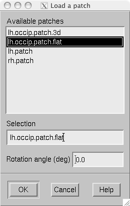
The patch selection dialog.
The main surface display has a section called Adjust view , which has the controls shown in Surface controls.:
L and R
Select the left or right hemisphere surface loaded through File/Load surface… .
B
Display the surfaces for both hemispheres.
M
Display the surfaces loaded File/Load morphing surface… according to the L, R, and B hemisphere selectors
P
Select the patch associated with the currently selected surface. For this to work, either L or R must be selected.
Option menu
Select one of the predefined view orientations, see Defining viewing orientations, below.
Arrow buttons
Rotate the surface by increments specified in degrees in the text box next to the arrows.
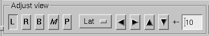
Surface controls.
The display can be also adjusted using keyboard shortcuts, which are available once you click in the main surface display with the left mouse button to make it active:
Arrow keys
Rotate the surface by increments specified in degrees in the Adjust View section.
+
Enlarge the image.
-
Reduce the image.
=
Return to the default size.
r
Rotate the image one full revolution around z axis using the currently specified rotation step. This is useful for producing a sequence of images when automatic image saving is on, see Producing output files.
s
Produces a raster image file which contains a snapshot of the currently displayed image. For information on snapshot mode, see Producing output files.
.
Stops the rotation invoked with the ‘r’ key, see above.
In addition, the mouse wheel or trackball can be used to rotate the image. If a trackball is available, e.g., with the Apple MightyMouse, the image can be rotated up and down or left and right with the trackball. With a mouse wheel the image will rotated up and down when the wheel is rotated. Image rotation in the left-right direction is achieved by holding down the shift key when rotating the wheel. The shift key has the same effect on trackball operation.
Note
The trackball and mouse wheel functionality is dependent on your X server settings. On Mac OSX these settings are normally correct by default but on a LINUX system some adjustments to the X server settings maybe necessary. Consult your system administrator or Google for details.
When you click on the surface with the left mouse button, the corresponding vertex number and the associated value will be displayed on the message line at the bottom of the display. In addition, the time course at this vertex will be shown, see Timecourses at vertices. You can also select a vertex by entering the vertex number to the text field at the bottom of the display. If the MRI viewer is displayed and Track surface location in MRI is selected in the MRI viewer control dialog, the cursor in the MRI slices will also follow the vertex selection, see Working with the MRI viewer.
The View menu choice Show coordinates… brings up a window which shows the coordinates of the selected vertex on the white matter surface, i.e., lh.white and rh.white FreeSurfer surfaces. If morphing surfaces have been loaded, the coordinates of both the subject being analyzed and those of the morphing subject will be shown. The Coordinates window includes the following lines:
MEG head
Indicates the vertex location in the MEG head coordinates. This entry will be present only if MEG/EEG data have been loaded.
Surface RAS (MRI)
Indicates the vertex location in the Surface RAS coordinates. This is the native coordinate system of the surfaces and this entry will always be present.
MNI Talairach
Shows the location in MNI Talairach coordinates. To be present, the MRI data of the subject must be in the mgz format (usually true with any recent FreeSurfer version) and the Talairach transformation must be appropriately defined during the FreeSurfer reconstruction workflow.
Talairach
Shows the location in the FreeSurfer Talairach coordinates which give a better match to the Talairach atlas.
The above coordinate systems are discussed in detail in MEG/EEG and MRI coordinate systems.
Note
By default, the tksurfer program, part of the FreeSurfer package, shows the vertex locations on the orig rather than white surfaces. Therefore, the coordinates shown in mne_analyze and tksurfer are by default slightly different (usually by < 1 mm). To make the two programs consistent, you can start tksurfer with the -orig white option.
The list of viewing orientations available in the Adjust View section of the main surface display is controlled
by a text file. The system-wide defaults reside in $MNE_ROOT/share/mne/mne_analyze/eyes .
If the file $HOME/.mne/eyes exists, it is used instead.
All lines in the eyes file starting with # are comments. The view orientation definition lines have the format:
<name>:<Left>:<Right>:<Left up>:<Right up> ,
where
<*name*>
is the name of this viewing orientation,
<*Left*>
specifies the coordinates of the viewing ‘eye’ location for the left hemisphere, separated by spaces,
<*Right*>
specifies the coordinates of the viewing location for the right hemisphere,
<*Left up*>
specifies the direction which is pointing up in the image for left hemisphere, and
<*Right up*>
is the corresponding up vector for the right hemisphere.
All values are given in a coordinate system where positive x points to the right, positive y to the front, and positive z up. The lengths of the vectors specified for each of the four items do not matter, since parallel projection is used and the up vectors will be automatically normalized. The up vectors are usually 0 0 1, i.e., pointing to the positive z direction unless the view is directly from above or below or if some special effect is desired.
The names of viewing orientations should be less than 9 characters long. Otherwise, the middle pane of the main display will not be able to accommodate all the controls. The widths of the main window panes can be adjusted from the squares at the vertical sashes separating the panes.
The scenes shown in the main surface display and the viewer, described in The viewer, are lit by fixed diffuse ambient lighting and a maximum of eight light sources. The states, locations, and colors of these light sources can be adjusted from the lighting adjustment dialog shown in The lighting adjustment dialog., which can be accessed through the Adjust/Lights… menu choice. The colors of the lights can be adjusted numerically or using a color adjustment dialog accessible through the Color… buttons.
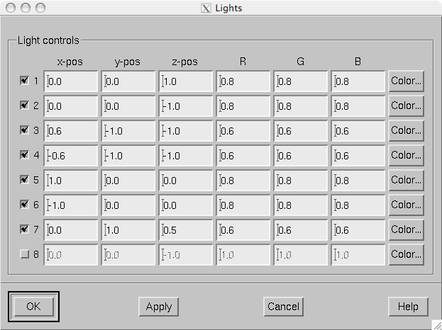
The lighting adjustment dialog.
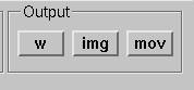
Graphics output controls.
Three types of output files can be produced from the main surface display using the graphics output buttons shown in Graphics output controls.:
w files (w button)
These files are simple binary files, which contain a list of vertex numbers on the cortical surface and their current data values. The w files will be automatically tagged with-lh.wand-rh.w. They will only contain vertices which currently have a nonzero value.
Graphics snapshots (img button)
These files will contain an exact copy of the image in tif or rgb formats. The output format and the output mode is selected from the image saving dialog shown in File type selection in the image saving dialog.. For more details, see Image output modes. If snapshot or automatic image saving mode is in effect, thee img button terminates this mode.
QuickTime (TM) movies (mov button)
These files will contain a sequence of images as a QuickTime (TM) movie file. The movie saving dialog shown in The controls in the movie saving dialog. specifies the time range and the interval between the frames as well as the quality of the movies, which is restricted to the range 25…100. The size of the QuickTime file produced is approximately proportional to the quality.
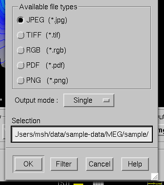
File type selection in the image saving dialog.
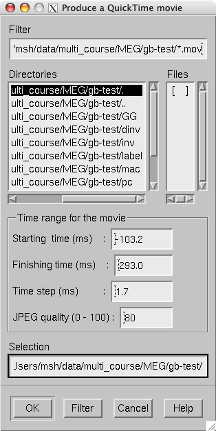
The controls in the movie saving dialog.
The image saving dialog shown in File type selection in the image saving dialog. selects the format of the image files produced and the image output mode. The buttons associated with different image format change the file name filter in the dialog to display files of desired type. However, the final output format is defined by the ending of the file name in the Selection text field as follows:
jpg
JPEG (Joint Photographic Experts Group) format. Best quality jpeg is always produced.
tif or tiff
Uncompressed TIFF (Tagged Image File Format).
rgb
RGB format.
Portable Document File format.
png
Portable Network Graphics format.
Note
Only TIFF and RGB output routines are compiled into mne_analyze . For other output formats to work, the following programs must be present in your system: tifftopdf, tifftopnm, pnmtojpeg, and pnmtopng.
There are three image saving modes which can be selected from the option menu labelled Output mode :
Single
When OK is clicked one file containing the present image is output.
Snapshot
A new image file is produced every timesis pressed in the image window, see Controlling the surface display and Overview. The image file name is used as the stem of the output files. For example, if the name is,sample.jpg, the output files will besample_shot_001.jpg,sample_shot_002.jpg, etc.
Automatic
A new image file is produced every time the image window changes. The image file name is used as the stem of the output files. For example, if the name is,sample.jpg, the output files will besample_001.jpg,sample_002.jpg, etc.
The displayed surface distributions can be morphed to another subject’s brain using the spherical morphing procedure, see Morphing and averaging. In addition to the morphing surfaces loaded through File/Load morphing surface… surface patches for the same subject can be loaded through File/Load morphing surface patch… . Switching between main and morphing surfaces is discussed in Controlling the surface display.
Any labels displayed are visible on any of the surfaces displayed in the main surface display. Time points can be picked in any of the surfaces. As a result, the corresponding timecourses will be shown in the MNE amplitude window, see Inquiring timecourses.
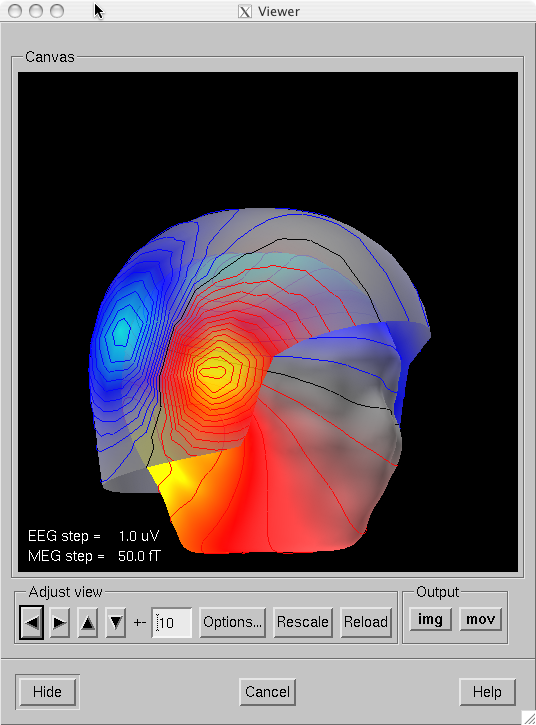
The viewer window with a visualization of MEG and EEG contour maps.
When Windows/Show viewer… is selected, the following additional surfaces will be loaded:
The scalp surface is loaded from the file bem/ <subject>“-head.fif“ under
the subject’s FreeSurfer directory. This surface is automatically
prepared if you use the watershed algorithm as described in Using the watershed algorithm.
If you have another source for the head triangulation you can use
the utility mne_surf2bem to create
the fif format scalp surface file, see Creating the BEM meshes.
If a file called bem/ <subject>“-bem.fif“ under
the subject’s FreeSurfer directory is present, mne_analyze tries
to load the BEM surface triangulations from there. This file can
be a symbolic link to one of the -bem.files created
by mne_prepare_bem_model , see Computing the BEM geometry data.
If the BEM file contains a head surface triangulation, it will be
used instead of the one present in the bem/ <subject>“-head.fif“ file.
Once all required surfaces have been loaded, the viewer window shown in The viewer window with a visualization of MEG and EEG contour maps. pops up. In addition to the display canvas, the viewer has Adjust view controls similar to the main surface display and options for graphics output. The Adjust view controls do not have the option menu for standard viewpoints and has two additional buttons:
The output options only include graphics output as snapshots (img ) or as movies (mov ).
Options…
This button pops up the viewer options window which controls the appearance of the viewer window.
Rescale
This button adjusts the contour level spacing in the magnetic field and electric potential contour maps so that the number of contour lines is reasonable.
Reload
Checks the modification dates of the surface files loaded to viewer and reloads the data if the files have been changed. This is useful, e.g., for display of different BEM tessellations.
The display can be also adjusted using keyboard shortcuts, which are available once you click in the viewer display with the left mouse button:
Arrow keys
Rotate the surface by increments specified in degrees in the Adjust View section.
+
Enlarge the image.
-
Reduce the image.
=
Return to the default size.
r
Rotate the image one full revolution around z axis using the currently specified rotation step. This is useful for producing a sequence of images when automatic image saving is on, see Producing output files.
s
Produces a image file which contains a snapshot of the currently displayed image. For information on snapshot mode, see Producing output files.
.
Stops the rotation invoked with the ‘r’ key, see above.
The left mouse button can be also used to inquire estimated magnetic field potential values on the helmet and head surfaces if the corresponding maps have been calculated and displayed.
In addition, the mouse wheel or trackball can be used to rotate the image. If a trackball is available, e.g., with the Apple MightyMouse, the image can be rotated up and down or left and right with the trackball. With a mouse wheel the image will rotated up and down when the wheel is rotated. Image rotation in the left-right direction is achieved by holding down the shift key when rotating the wheel. The shift key has the same effect on trackball operation.
Note
The trackball and mouse wheel functionality is dependent on your X server settings. On Mac OSX these settings are normally correct by default but on a LINUX system some adjustments to the X server settings maybe necessary. Consult your system administrator or Google for details.
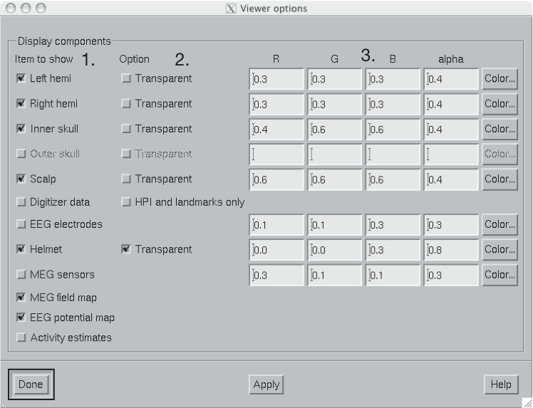
The viewer options window
The viewer options window shown above contains three main sections to control the appearance of the viewer:
The available items are:
Left hemi
The pial surface of the left hemisphere. This surface can be made transparent. Naturally, this surface will only be visible if the scalp is made transparent.
Right hemi
The pial surface of the right hemisphere.
Inner skull
The inner skull surface. This surface can be made transparent. If parts of the pial surface are outside of the inner skull surface, they will be visible, indicating that the inner skull surface is obviously inside the inner skull. Note that this criterion is more conservative than the one imposed during the computation of the forward solution since the source space points are located on the white matter surface rather than on the pial surface. This surface can be displayed only if the BEM file is present, see Overview.
Outer skull
The outer skull surface. This surface can be made transparent. This surface can be displayed only if the BEM file is present and contains the outer skull surface, see Overview.
Scalp
The scalp surface. This surface can be made transparent. The display of this surface requires that the scalp triangulation file is present, see Overview.
Digitizer data
The 3D digitizer data collected before the MEG/EEG acquisition. These data are loaded from File/Load digitizer data… . The display can be restricted to HPI coil locations and cardinal landmarks with the option. The digitizer points are shown as disks whose radius is equal to the distance of the corresponding point from the scalp surface. Points outside the scalp are shown in red and those inside in blue. Distinct shades of cold and warm colors are used for the fiducial landmarks. The HPI coils are shown in green. Further information on these data and their use in coordinate system alignment is given in Coordinate frame alignment.
Helmet
The MEG measurement surface, i.e., inner surface of the dewar.
EEG electrodes
The EEG electrode locations. These will be only available if your data set contains EEG channels.
MEG sensors
Outlines of MEG sensors.
MEG field map
Estimated contour map of the magnetic field component normal to the helmet surface or normal to the scalp, see Magnetic field and electric potential maps.
EEG potential map
Interpolated EEG potential map on the scalp surface, see Magnetic field and electric potential maps.
Activity estimates
Current estimates on the pial surface.
In mne_analyze , the magnetic field and potential maps displayed in the viewer window are computed using an MNE-based interpolation technique. This approach involves the following steps:
The magnetic field and potential maps appear automatically whenever they are enabled from the viewer options, see Viewer options.
Let \(x_k\) be an MEG or an EEG signal at channel \(k = 1 \dotso N\). This signal is related to the primary current distribution \(J^p(r)\) through the lead field \(L_k(r)\):
where the integration space \(G\) in our case is a spherical surface. The oblique boldface characters denote three-component locations vectors and vector fields.
The inner product of two leadfields is defined as:
These products constitute the Gram matrix \(\Gamma_{jk} = \langle L_j \mid L_k \rangle\). The minimum -norm estimate can be expressed as a weighted sum of the lead fields:
where \(w\) is a weight vector and \(L\) is a vector composed of the continuous lead-field functions. The weights are determined by the requirement
i.e., the estimate must predict the measured signals. Hence,
However, the Gram matrix is ill conditioned and regularization must be employed to yield a stable solution. With help of the SVD
a regularized minimum-norm can now found by replacing the data matching condition by
where
respectively. In the above, the columns of \(U^{(p)}\) are the first k left singular vectors of \(\Gamma\). The weights of the regularized estimate are
where \(\Lambda^{(p)}\) is diagonal with
\(\lambda_j\) being the \(j\) th singular value of \(\Gamma\). The truncation point \(p\) is selected in mne_analyze by specifying a tolerance \(\varepsilon\), which is used to determine \(p\) such that
The extrapolated and interpolated magnetic field or potential distribution estimates \(\hat{x'}\) in a virtual grid of sensors can be now easily computed from the regularized minimum-norm estimate. With
where \(L_j'\) are the lead fields of the virtual sensors,
The parameters of the field maps can be adjusted from the Field mapping preferences dialog shown in Field mapping preferences dialog. which is accessed through the Adjust/Field mapping… menu item.
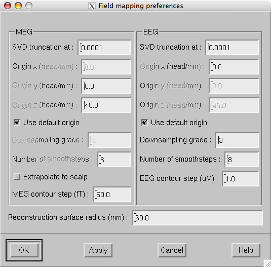
Field mapping preferences dialog.
The Field mapping preferences dialog has the following controls, arranged in MEG , EEG , and common sections:
SVD truncation at
Adjusts the smoothing of the field and potential patterns. This parameter specifies the eigenvalue truncation point as described in Technical description. Smaller values correspond to noisier field patterns with less smoothing.
Use default origin
The location of the origin of the spherical head model used in these computations defaults to (0 0 40) mm. If this box is unchecked the origin coordinate fields are enabled to enter a custom origin location. Usually the default origin is appropriate.
Downsampling grade
This option only applies to EEG potential maps and MEG field maps extrapolated to the head surface and controls the number of virtual electrodes or point magnetometers used in the interpolation. Allowed values are: 2 (162 locations), 3 (642 locations), and 4 (2562 locations). Usually the default value 3 is appropriate.
Number of smoothsteps
This option controls how much smoothing, see About smoothing, is applied to the interpolated data before computing the contours. Usually the default value is appropriate.
Reconstruction surface radius
Distance of the spherical reconstruction surface from the sphere model origin. Usually default value is appropriate. For children it may be necessary to make this value smaller.
The characteristics of the current estimates displayed are controlled from the MNE preferences dialog which pops up from Adjust/Estimates… .
This dialog, shown in Estimate preferences dialog., has the following controls:
SNR estimate
This controls the regularization of the estimate, i.e., the amount of allowed mismatch between the measured data and those predicted by the estimated current distribution. Smaller SNR means larger allowed mismatch. Typical range of SNR values is 1…7. As discussed in Minimum-norm estimates, the SNR value can be translated to the current variance values expressed in the source-covariance matrix R. This translation is presented as the equivalent current standard-deviation value
Show
This radio button box selects the quantity to display. MNE is the minimum norm estimate (estimated value of the current), dSPM is the noise-normalized MNE, and sLORETA is another version of the noise-normalized solution which is claimed to have a smaller location bias than the dSPM.
Mask with
If MNE is selected in the Show radio button box, it is possible to mask the solution with one of the statistical maps. The masking map is thresholded at the value given in the Threshold text field and the MNE is only shown in areas with statistical values above this threshold.
Value histogram
This part of the dialog shows the distribution of the currently shown estimate values over the surface. The histogram is colored to reflect the current scale settings. The fthresh , fmid , and fmax values are indicated with vertical bars. The histogram is updated when the dialog is popped up and when the estimate type to show changes, not at every new time point selection. The Refresh button makes the histogram current at any time.
Color scale
These text fields control the color scale as described in The color scale parameters..
Options
Various options controlling the estimates.
| Parameter | Meaning |
|---|---|
| fthresh | If the value is below this level, it will not be shown. |
| fmid | Positive values at this level will show as red. Negative values will be dark blue. |
| fmax | Positive values at and above this level will be bright yellow. Negative values will be bright blue. |
| fmult | Apply this multiplier to the above thresholds. Default is \(1\) for statistical maps and \(1^{-10}\) for currents (MNE). The vertical bar locations in the histogram take this multiplier into account but the values indicated are the threshold parameters without the multiplier. |
| tcmult | The upper limit of the timecourse vertical scale will be \(tc_{mult}f_{mult}f_{max}\). |
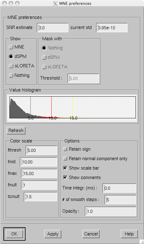
Estimate preferences dialog.
The optional parameters are:
Retain sign
With this option, the sign of the dot product between the current direction and the cortical surface normal will be used as the sign of the values to be displayed. This option yields meaningful data only if a strict or a loose orientation constraint was used in the computation of the inverse operator decomposition.
Retain normal component only
Consider only the current component normal to the cortical mantle. This option is not meaningful with completely free source orientations.
Show scale bar
Show the color scale bar at the lower right corner of the display.
Show comments
Show the standard comments at the lower left corner of the display.
Time integr. (ms)
Integration time for each frame (\(\Delta t\)). Before computing the estimates time integration will be performed on sensor data. If the time specified for a frame is \(t_0\), the integration range will be \(t_0 - ^{\Delta t}/_2 \leq t \leq t_0 + ^{\Delta t}/_2\).
# of smooth steps
Before display, the data will be smoothed using this number of steps, see About smoothing.
Opacity
The range of this parameter is 0…1. The default value 1 means that the map overlaid on the cortical surface is completely opaque. With lower opacities the color of the cortical surface will be visible to facilitate understanding the underlying folding pattern from the curvature data displayed.
The SNR estimate display shows the SNR estimated from the whitened data in red and the apparent SNR inferred from the mismatch between the measured and predicted data in green.
The SNR estimate is computed from the whitened data \(\tilde{x}(t)\), related to the measured data \(x(t)\) by
where \(C^{-^1/_2}\) is the whitening operator, introduced in Whitening and scaling.
The computation of the apparent SNR will be explained in future revisions of this manual.
Timecourses at individual vertices can be inquired by clicking on a desired point on the surface with the left mouse button. If the control key was down at the time of a click, the timecourse will be added to the timecourse manager but left off. With both control and shift down, the timecourse will be added to the timecourse manager and switched on. For more information on the timecourse manager, see The timecourse manager.
The timecourses are be affected by the Retain sign and Retain normal component only settings in the MNE preferences dialog , see Preferences.
The labels provide means to interrogate timecourse information
from ROIs. The label files can be created in mne_analyze ,
see Creating new label files or in tksurfer ,
which is part of the FreeSurfer software. For mne_analyze left-hemisphere
and right-hemisphere label files should be named <name> -lh.label and <name> -rh.label ,
respectively.
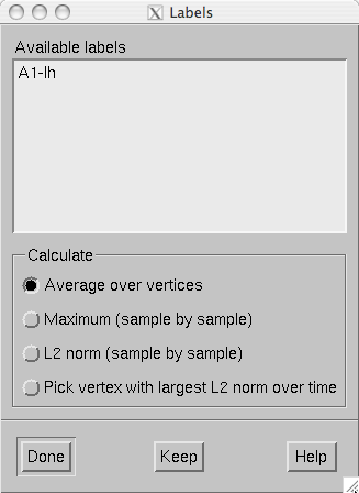
Individual label files can be loaded from Labels/Load label… . All label files in a directory can be loaded from Labels/Load all labels… . Once labels are loaded, the label list shown in The label list. appears. Each time a new label is added to the list, the names will be reordered to alphabetical order. This list can be also brought up from Labels/Show label list . The list can be cleared from Labels/Discard all labels .
Warning
Because of the format of the label files mne_analyze can not certify that the label files loaded belong to the cortical surfaces of the present subject.
When a label is selected from the label list, the corresponding timecourse appears. The Keep button stores the timecourse to the timecourse manager, The timecourse manager.
The label list.
The timecourse shown in the MNE amplitude window is a compound measure of all timecourses within a label. Two measures are available:
Average
Compute the average over all label vertices at each time point.
Maximum
Compute the maximum absolute value over all vertices at each time point. If the data are signed, the value is assigned the sign of the value at the maximum vertex. This may make the timecourse jump from positive to negative abruptly if vertices with different signs are included in the label.
L2 norm (sample by sample)
Compute the \(l_2\) norm over the values in the vertices at each time point.
Pick vertex with largest L2 norm over time
Compute the \(l_2\) norm over time in each vertex and show the time course at the vertex with the largest norm.
The timecourse manager shown in The timecourse manager. has the following controls for each timecourse stored:
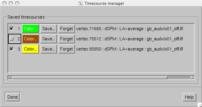
The timecourse manager.
Numbered checkbox
Switches the display of this timecourse on and off.
Color…
This button shows the color of the timecourse curve. The color can be adjusted from the color editor which appears when the button is pressed.
Save…
Saves the timecourse. If a single vertex is selected, the time course file will contain some comment lines starting with the the percent sign, one row of time point values in seconds and another with the data values. The format of the timecourse data is explained in Label timecourse files, below.
Forget
Delete this timecourse from memory.
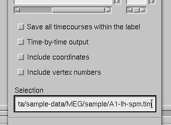
When timecourse corresponding to a label is saved, the default is to save the displayed single timecourse in a format identical to the vertex timecourses. If Save all timecourses within the label is selected, the Time-by-time output output changes the output to be listed time by time rather than vertex by vertex, Include coordinates adds the vertex location information to the output file, and Include vertex numbers adds the indices of picked vertices to the output, see Label timecourse saving options.. The vertex-by-vertex output formats is summarized in Vertex-by-vertex output format. is the number of vertices, is the number of time points, is the number of comment lines, indicate the times in milliseconds, is a vertex number, are the coordinates of vertex in millimeters, and are the values at vertex . Items in brackets are only included if Include coordinates is active. In the time-by-time output format the data portion of the file is transposed..
Label timecourse saving options.
| Line | Contents |
|---|---|
| \(1-n_{com}\) | Comment lines beginning with % |
| \(n_{com}+1\) | \(\{0.0\}[0.0\ 0.0\ 0.0] t_1 \dotso t_{n_t}\) |
| \((n_{com}+1)-(n_p+n_{com}+1)\) | \(\{p\}[x_p y_p z_p]v_p^{(1)} \dotso v_p^{(n_t)}\) |
It is easy to create new label files in mne_analyze. For this purpose, an inflated surface should be visible in the main display. Follow these steps:
-lh.label or -rh.label ,
depending on the hemisphere on which the label is specified.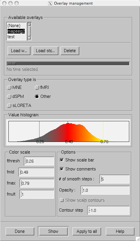
The overlay management dialog.
In addition to source estimates derived from MEG and EEG data, mne_analyze can be used to display other surface-based data. These overlay data can be imported from w and stc files containing single time slice (static) and dynamic data (movies), respectively. These data files can be produced by mne_make_movie , FreeSurfer software, and custom programs or Matlab scripts.
The names of the files to be imported should end with - <hemi> .<type> , where <hemi> indicates
the hemisphere (lh or rh and <type> is w or stc .
Overlays are managed from the dialog shown in The overlay management dialog. which is invoked from File/Manage overlays… .
This dialog contains the following controls:
List of overlays loaded
Lists the names of the overlays loaded so far.
Load w…
Load a static overlay from a w file. In the open dialog it is possible to specify whether this file contains data for the cortical surface or for scalp. Scalp overlays can be viewed in the viewer window.
Load stc…
Load a dynamic overlay from an stc file. In the open dialog it is possible to specify whether this file contains data for the cortical surface or for scalp. Scalp overlays can be viewed in the viewer window.
Delete
Delete the selected overlay from memory.
Time scale slider
Will be activated if a dynamic overlay is selected. Changes the current time point.
Overlay type is
Selects the type of the data in the current overlay. Different default color scales are provided each overlay type.
Value histogram
Shows the distribution of the values in the current overlay. For large stc files this may take a while to compute since all time points are included. The histogram is colored to reflect the current scale settings. The fthresh , fmid , and fmax values are indicated with vertical bars.
Color scale
Sets the color scale of the current overlay. To activate the values, press Show . For information on color scale settings, see The color scale parameters..
Options
Display options. This a subset of the options in the MNE preferences dialog. For details, see Preferences.
Show
Show the selected overlay and assign the settings to the current overlay.
Apply to all
Apply the current settings to all loaded overlays.
It is also possible to inquire timecourses of vertices and labels from dynamic (stc) cortical overlays in the same way as from original data and store the results in text files. If a static overlay (w file) or a scalp overlay is selected, the timecourses are picked from the data loaded, if available.
Starting from MNE software version 2.6, mne_analyze includes routines for fitting current dipoles to the data. At present mne_analyze is limited to fitting single equivalent current dipole (ECD) at one time point. The parameters affecting the dipole fitting procedure are described in Dipole fitting parameters. The results are shown in the dipole list (The dipole list). The selection of channels included can be adjusted interactively or by predefined selections as described in Channel selections.
Warning
The current dipole fitting has been added recently and has not been tested comprehensively. Especially fitting dipoles to EEG data may be unreliable.
Prior to fitting current dipoles, the fitting parameters must be set with the Dipole fitting preferences dialog shown in The dipole fitting preferences dialog.. The dialog is brought up from the Setup fitting… choice in the Dipoles menu. This dialog contains three sections: Forward model , Modalities , and Noise estimate .
The Forward model section specifies the forward model to be used:
Sphere model origin x/y/z [mm]
Specifies the origin of the spherically symmetric conductor model in MEG/EEG head coordinates, see The head and device coordinate systems.
EEG scalp radius [mm]
Specifies the radius of the outermost shell in the EEG sphere model. For details, see The EEG sphere model definition file.
EEG sphere model name
Specifies the name of the EEG sphere model to use. For details, see The EEG sphere model definition file.
BEM model
Selects the boundary-element model to use. The button labeled with … brings up a file-selection dialog to select the BEM file. An existing selection can be cleared with the Unset button. If EEG data are included in fitting, this must be a three-compartment model. Note that the sphere model is used even with a BEM model in effect, see The dipole fitting algorithm.
Accurate field calculation
Switches on the more accurate geometry definition of MEG coils, see Coil geometry information. In dipole fitting, there is very little difference between the accurate and normal coil geometry definitions.
The Modalities section defines which kind of data (MEG/EEG) are used in fitting. If an inverse operator is loaded with the data, this section is fixed and greyed out. You can further restrict the selection of channels used in dipole fitting with help of channel selections discussed in Channel selections.
The Noise estimate section of the dialog contains the following items:
Noise covariance
Selects the file containing the noise-covariance matrix. If an inverse operator is loaded, the default is the inverse operator file. The button labeled with … brings up a file-selection dialog to select the noise covariance matrix file. An existing selection can be cleared with the Unset button.
Omit off-diagonal terms
If a noise covariance matrix is selected, this choice omits the off-diagonal terms from it. This means that individual noise estimates for each channel are used but correlations among channels are not taken into account.
Regularization
Regularize the noise covariance before using it in whitening by adding a multiple of an identity matrix to the diagonal. This is discussed in more detail in Regularization of the noise-covariance matrix. Especially if EEG is included in fitting it is advisable to enter a non-zero value (around 0.1) here.
Planar fixed [fT/cm]
In the absence of a noise covariance matrix selection, a diagonal noise covariance with fixed values on the diagonal is used. This entry specifies the fixed value of the planar gradiometers.
Axial fixed [fT]
If a noise covariance matrix file is not specified, this entry specifies a fixed diagonal noise covariance matrix value for axial gradiometers and magnetometers.
EEG fixed [muV]
If a noise covariance matrix file is not specified, this entry specifies a fixed diagonal noise covariance matrix value for axial gradiometers and magnetometers..
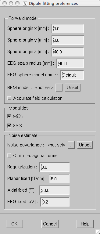
The dipole fitting preferences dialog.
When the dipole fitting preferences dialog is closed and the values have been modified the following preparatory calculations take place:
When the Fit ECD button in the tool bar is clicked with a time point selected from the the response, the optimal Equivalent Current Dipole parameters (location, orientation, and amplitude) are determined using the following algorithm:
Additional notes:
mne_dipole_fit --help lists the command-line options which have direct correspondence
to the interactive dipole fitting options discussed here.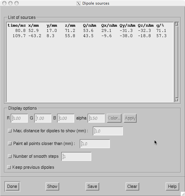
The dipole list.
The dipole list dialog shown in The dipole list. contains the parameters of the dipoles fitted. In addition, it is possible to import current dipole locations from the Neuromag source modelling program xfit to mne_analyze . Dipoles can be imported in two ways:
The buttons at the bottom of the dialog perform the following functions:
Done
Hide the dialog.
Show
Show the currently selected dipoles as specified in Display options , see below.
Save
Save the selected (or all) dipoles. If the file name specified in the file selection dialog that pops up ends with.bdip, the dipole data will be saved in the binary bdip format compatible with the Neuromag xfit software, otherwise, a text format output will be used. In the text file, comments will be included on lines starting with the percent sign so that the text format can be easily loaded into Matlab.
Clear
Clear the selected dipoles from the list.
When you double click on one of the dipoles or select several dipoles and click Show points on the surface displayed in the vicinity of the dipoles will be painted according to the specifications given in the Options section of the dialog:
Color
By the default, the dipoles are marked in green with transparency (alpha) set to 0.5. I you click on one of the dipoles, you can adjust the color of this dipole by editing the color values or from the color editor appearing when you click Color… . When you click Apply , the new color values are attached to the selected dipole.
Max. distance for dipoles to show (mm)
If this option is on, only dipoles which are closer to the surface than the distance specified in the adjacent text field are displayed.
Paint all point closer than (mm)
Instead of indicating the point closest to the dipole all points closer than the distance given in the text field will be painted if this option is on. This choice is useful for understanding the shape of the neighborhood of a dipole on the cortical surface.
Number of smooth steps
This option spreads out the dipole marking by the given number of smooth steps to make the dipoles more clearly visible. A suitable choice is 3 or 4.
Keep previous dipoles
If this option is on, previously marked dipoles are not cleared from the display before new ones are shown.
Note
The surface must be loaded to display dipole locations. To calculate the distance from the dipoles to the white matter surface, the white matter tessellation is loaded as needed. Depending on the precise location of the fitted dipole, the spot indicating the dipole site may easily appear on a different wall of a fissure than could be expected. The fissural walls can be far apart from each other in the inflated view of the cortex even if they are physically separated by just a few millimeters. The size of the spots indicating the dipole locations do not relate to the dipole strengths or their confidence limits in any way.
As mentioned in The topographical display, the right mouse button in the topographical display of channels can be used to restrict the selection of channels taken into account in dipole fitting. In addition, the channel selections can be manipulated in the channel selection window, which pops up from Dipoles/Manage channel selections… . Initially this dialog contains the selections defined in or $HOME/.mne/mne_analyze.sel or $MNE_ROOT/share/mne/mne_analyze/mne_analyze.sel, the personal file taking precedence over the system wide default. The Save button in this dialog save the current set of channel selections to the personal selection file. The format of this file is identical to the channel selection file in mne_browse_raw .
When a channel selection file is in effect. the variances of the unselected channels are increased by a factor of 900. This means that unselected channels receive virtually no weight in the least-squares error function or, equivalently, that they are considered to be 30 times more noisy than their true noise value. Since this implementation of channel selections requires recomputation of the initial guess candidate data discussed in The dipole fitting algorithm, above, changing the selection may take a finite amount of time, especially if a BEM is used for the forward calculation.
Note
Please note that when making a channel selection in the topographical displays, the channels not present in a particular layout are also affected. For example, if you select channels in a layout showing the Vectorview planar gradiometers, the magnetometer channels and EEG channels will be unselected.
The MRI-MEG coordinate frame alignment tools included in mne_analyze utilized the 3D digitizer (Polhemus) data acquired in the beginning of each MEG/EEG session and the scalp surface triangulation shown in the viewer window. To access the coordinate frame alignment tools:
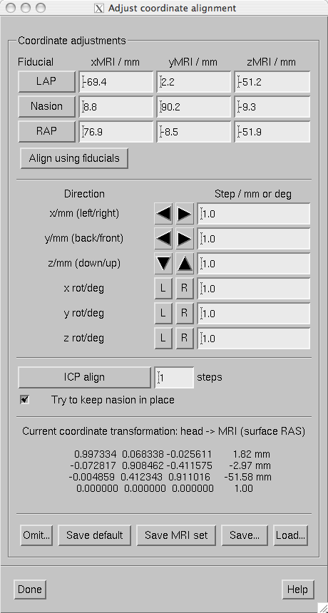
The coordinate frame alignment dialog.
The coordinate frame alignment dialog contains the following sections:
The saving and loading choices are:
Save default
Saves a file which contains the MEG/MRI coordinate transformation only. The file name is generated from the name of the file from which the digitization data were loaded by replacing the ending.fifwith-trans.fif. If this file already exists, it will be overwritten without any questions asked.
Save MRI set
This option searches for a file called COR.fif in $SUBJECTS_DIR/$SUBJECT/mri/T1-neuromag/sets. The file is copied to COR-<username>-<date>-<time>.fif and the current MEG/MRI coordinate transformation as well as the fiducial locations in MRI coordinates are inserted.
Save…
Saves a file which contains the MEG/MRI coordinate transformation only. The ending-trans.fifis recommended. The file name selection dialog as a button to overwrite.
Load…
Loads the MEG/MRI coordinate transformation from the file specified.
The MEG/MRI coordinate transformation files are employed in the forward calculations. The convenience script mne_do_forward solution described in Computing the forward solution uses a search sequence which is compatible with the file naming conventions described above. It is recommended that -trans.fif file saved with the Save default and Save… options in the mne_analyze alignment dialog are used because then the $SUBJECTS_DIR/$SUBJECT directory will be composed of files which are dependent on the subjects’s anatomy only, not on the MEG/EEG data to be analyzed.
Each iteration step of the Iterative Closest Point (ICP) algorithm consists of two matching procedures:
These two steps are iterated the designated number of times. If the Try to keep nasion in place option is on, the present location of the nasion receives a strong weight in the second part of each iteration step so that nasion movements are discouraged.
Note
One possible practical approach to coordinate frame alignment is discussed in MEG-MRI coordinate system alignment.
The newest version of FreeSurfer contains a script called mkheadsurf which
can be used for coordinate alignment purposes. For more information,
try mkheadsurf --help . This script produces a file
called surf/lh.smseghead , which can be converted into
a fif file using mne_surf2bem.
Suggested usage:
mkheadsurf -subjid <subject> .$SUBJECTS_DIR/ <subject> /bem .mne_surf2bem --surf ../surf/lh.smseghead --id 4 --check --fif <subject> -head-dense.fif-head-sparse.fif-head-dense.fif to <subject> -head.fifAfter this you can switch between the dense and smooth head
surface tessellations by copying either <subject> -head-dense.fif or <subject> -head-sparse.fif to <subject> -head.fif .
If you have Matlab software available on your system, you
can also benefit from the script mne_make_scalp_surfaces .
This script invokes mkheadsurf and
subsequently decimates it using the mne_reduce_surface function
in the MNE Matlab toolbox, which in turn invokes the reducepatch
Matlab function. As a result, the $SUBJECTS_DIR/$SUBJECT/bem directory
will contain ‘dense’, ‘medium’,
and ‘sparse’ scalp surface tessellations. The
dense tessellation contains the output of mkheadsurf while
the medium and sparse tessellations comprise 30,000 and 2,500 triangles,
respectively. You can then make a symbolic link of one of these
to <subject> -head.fif .
The medium grade tessellation is an excellent compromize between
geometric accuracy and speed in the coordinate system alignment.
Note
While the dense head surface tessellation may help in coordinate frame alignment, it will slow down the operation of the viewer window considerably. Furthermore, it cannot be used in forward modelling due to the huge number of triangles. For the BEM, the dense tessellation does not provide much benefit because the potential distributions are quite smooth and widespread on the scalp.
If you have identified the three fiducial points in software outside mne_analyze , it is possible to display this information on the head surface visualization. To do this, you need to copy the file containing the fiducial location information in MRI (surface RAS) coordinates to $SUBJECTS_DIR/$SUBJECT/bem/$SUBJECT-fiducials.fif. There a three supported ways to create this file:
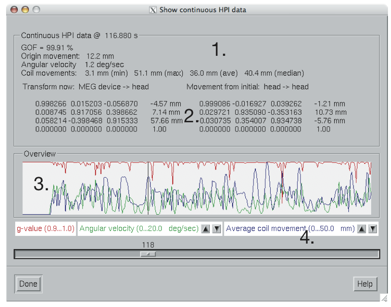
Continuous HPI data overview.
The newest versions of Neuromag software allow continuous acquisition of signals from the HPI coils. On the basis of these data the relative position of the dewar and the head can be computed a few times per second. The resulting location data, expressed in the form of unit quaternions (see http://en.wikipedia.org/wiki/Quaternion) and a translation.
The continuous HPI data can be through the File/View continuous HPI data… menu item, which pops up
a standard file selection dialog. If the file specified ends with .fif a
fif file containing the continuous coordinate transformation information
is expected. Otherwise, a text log file is read. Both files are
produced by the Neuromag maxfilter software.
Once the data have been successfully loaded, the dialog shown in Continuous HPI data overview. appears. It contains the following information:
The overview items are:
GOF
Geometric mean of the goodness of fit values of the HPI coils at this time point.
Origin movement
The distance between the head coordinate origins at the first and current time points.
Angular velocity
Estimated current angular velocity of the head.
Coil movements
Comparison of the sensor locations between the first and current time points. The minimum, maximum, average, and median sensor movements are listed.
The graphical display contains the following data:
The slider below the display can be used to select the time point. If you click on the slider, the current time can be adjusted with the arrow keys. The current head position with respect to the sensor array is show in the viewer window if it is visible, see The viewer. Note that a complete set of items listed above is only available if a data file has been previously loaded, see Loading data.
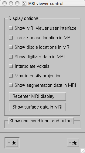
The MRI viewer control window.
Selecting Show MRI viewer… from the View menu starts the FreeSurfer MRI viewer program tkmedit to work in conjunction with mne_analyze . After a few moments, both tkmedit with the current subject’s T1 MRI data shown and the MRI viewer control window shown in The MRI viewer control window. appear. Note that the tkmedit user interface is initially hidden. The surfaces of a subject must be loaded before starting the MRI viewer.
The MRI viewer control window contains the following items:
Show MRI viewer user interface
If this item is checked, the tkmedit user interface window will be show.
Track surface location in MRI
With this item checked, the cursor in the MRI data window follows the current (clicked) location in surface display or viewer. Note that for the viewer window the surface location will inquired from the surface closest to the viewer. The MEG helmet surface will not be considered. For example, if you click at an EEG electrode location with the scalp surface displayed, the location of that electrode on the scalp will be shown. The cortical surface locations are inquired from the white matter surface.
Show dipole locations in MRI
If this option is selected, whenever a dipole is displayed in the surface view using the dipole list dialog discussed in The dipole list the cursor will also move to the same location in the MRI data window.
Show digitizer data in MRI
If digitizer data are loaded, this option shows the locations with green diamonds in the MRI data.
Interpolate voxels
Toggles trilinear interpolation in the MRI data on and off.
Max. intensity projection
Shows a maximum-intensity projection of the MRI data. This is useful in conjunction with the Show digitizer data in MRI option to evaluate the MEG/MRI coordinate alignment
Recenter MRI display
Brings the cursor to the center of the MRI data.
Show surface data in MRI
This button creates an MRI data set containing the surface data displayed and overlays in with the MRI slices shown in the MRI viewer.
Show segmentation data in MRI
If available, the standard automatically generated segmentation volume (mri/aparc+aseg) is overlaid on the MRI using the standard FreeSurfer color lookup table ($FREESURFER_HOME/FreeSurferColorLUT.txt). As a result, the name of the brain structure or region of corex at the current location of the cursor will be reported if the tkmedit user interface is visible. After the segmentation is loaded this button toggles the display of the segmentation on and off.
Show command input and output
Allows sending tcl commands to tkmedit and shows the responses received. The tkmedit tcl scripting commands are discussed at https://surfer.nmr.mgh.harvard.edu/fswiki/TkMeditGuide/TkMeditReference/TkMeditScripting.
The FreeSurfer software includes an average subject (fsaverage) with a cortical surface reconstruction. In some cases, the average subject can be used as a surrogate if the MRIs of a subject are not available.
The MNE software comes with additional files which facilitate the use of the average subject in conjunction with mne_analyze . These files are located in the directory $MNE_ROOT/mne/setup/mne_analyze/fsaverage:
fsaverage_head.fif
The approximate head surface triangulation for fsaverage.
fsaverage_inner_skull-bem.fif
The approximate inner skull surface for fsaverage.
fsaverage-fiducials.fif
The locations of the fiducial points (LPA, RPA, and nasion) in MRI coordinates, see Using fiducial points identified by other software.
fsaverage-trans.fif
Contains a default MEG-MRI coordinate transformation suitable for fsaverage. For details of using the default transformation, see Loading data.
The following graphics displays are compatible with the Elekta-Neuromag report composer cliplab :
The graphics can be dragged and dropped from these windows to one of the cliplab view areas using the middle mouse button. Because the topographical display area has another function (bed channel selection) tied to the middle mouse button, the graphics is transferred by doing a middle mouse button drag and drop from the label showing the current time underneath the display area itself.
Note
The cliplab drag-and-drop functionality requires that you have the proprietary Elekta-Neuromag analysis software installed. mne_analyze is compatible with cliplab versions 1.2.13 and later.
When mne_analyze is invoked
with the --visualizehpi option, a simplified user interface shown
in Snapshot of mne_analyze in the head position visualization mode. is displayed. This interface consists only
of the viewer window. This head position visualization mode
can be used with existing data files but is most useful for showing
immediate feedback of the head position during experiments with
an Elekta-Neuromag MEG system.
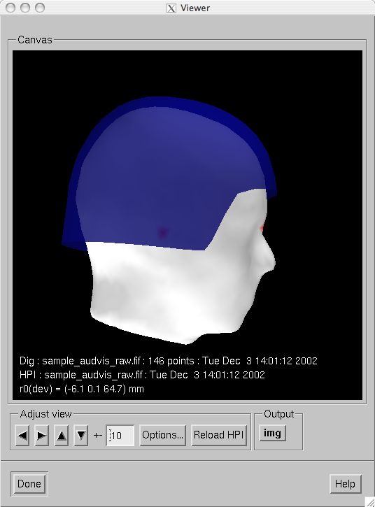
Snapshot of mne_analyze in the head position visualization mode.
As described in mne_analyze, the head position visualization mode can be customized with the –dig, –hpi, –scalehead, and –rthelmet options. For this mode to be useful, the –dig and –hpi options are mandatory. If existing saved data are viewed, both of these can point to a average or raw data file. For on-line operation with the Elekta-Neuromag systems, the following files in should be used:
--dig /neuro/dacq/meas_info/isotrak --hpi /neuro/dacq/meas_info/hpi_result
Note
Since MNE software runs only on LINUX and Mac OS X platforms, one usually needs to NFS mount the volume containing /neuro directory to another system and access these files remotely. However, Neuromag has indicated that future versions of their acquisition software will run on the LINUX platform as well and the complication of remote operation can then be avoided.
When mne_analyze starts in the head position visualization mode and the –dig and –hpi options have been specified, the following sequence operations takes place:
--scalehead option is invoked, the average head surface
is scaled to the approximate size of the subject’s head
by fitting a sphere to the digitizer and to the head surface points
lying above the plane of the fiducial landmarks, respectively. The
standard head surface is then scaled by the ration of the radiuses
of these two best-fitting spheres. Without –scalehead, the standard
head surface is used as is without scaling.If the --rthelmet option was present, the room-temperature
helmet surface is shown instead of the MEG sensor surface. The digitizer
and HPI data files are reloaded and the above steps 1. - 4. are
repeated when the Reload HPI button
is pressed. The comment lines in the viewer window show information
about the digitizer and HPI data files as well as the location of the
MEG device coordinate origin in the MEG head coordinate system.
Note
The appearance of the viewer visualization can be customized using the Options… button, see Viewer options. Since only the scalp and MEG device surfaces are loaded, only a limited number of options is active. The display can also be saved as an image from the img button, see Producing output files.