import os.path as op
import numpy as np
import matplotlib.pyplot as plt

import mne
In this tutorial we focus on plotting functions of mne.Evoked.
First we read the evoked object from a file. Check out
Epoching and averaging (ERP/ERF) to get to this stage from raw data.
data_path = mne.datasets.sample.data_path()
fname = op.join(data_path, 'MEG', 'sample', 'sample_audvis-ave.fif')
evoked = mne.read_evokeds(fname, baseline=(None, 0), proj=True)
print(evoked)
Out:
Reading /home/ubuntu/mne_data/MNE-sample-data/MEG/sample/sample_audvis-ave.fif ...
    Read a total of 4 projection items:
        PCA-v1 (1 x 10²) active
        PCA-v2 (1 x 10²) active
        PCA-v3 (1 x 10²) active
        Average EEG reference (1 x 60) active
    Found the data of interest:
        t =    -199.80 ...     499.49 ms (Left Auditory)
        0 CTF compensation matrices available
        nave = 55 - aspect type = 100
Projections have already been applied. Setting proj attribute to True.
Applying baseline correction (mode: mean)
    Read a total of 4 projection items:
        PCA-v1 (1 x 10²) active
        PCA-v2 (1 x 10²) active
        PCA-v3 (1 x 10²) active
        Average EEG reference (1 x 60) active
    Found the data of interest:
        t =    -199.80 ...     499.49 ms (Right Auditory)
        0 CTF compensation matrices available
        nave = 61 - aspect type = 100
Projections have already been applied. Setting proj attribute to True.
Applying baseline correction (mode: mean)
    Read a total of 4 projection items:
        PCA-v1 (1 x 10²) active
        PCA-v2 (1 x 10²) active
        PCA-v3 (1 x 10²) active
        Average EEG reference (1 x 60) active
    Found the data of interest:
        t =    -199.80 ...     499.49 ms (Left visual)
        0 CTF compensation matrices available
        nave = 67 - aspect type = 100
Projections have already been applied. Setting proj attribute to True.
Applying baseline correction (mode: mean)
    Read a total of 4 projection items:
        PCA-v1 (1 x 10²) active
        PCA-v2 (1 x 10²) active
        PCA-v3 (1 x 10²) active
        Average EEG reference (1 x 60) active
    Found the data of interest:
        t =    -199.80 ...     499.49 ms (Right visual)
        0 CTF compensation matrices available
        nave = 58 - aspect type = 100
Projections have already been applied. Setting proj attribute to True.
Applying baseline correction (mode: mean)
[<Evoked  |  comment : 'Left Auditory', kind : average, time : [-0.199795, 0.499488], n_epochs : 55, n_channels x n_times : 376 x 421, ~4.9 MB>, <Evoked  |  comment : 'Right Auditory', kind : average, time : [-0.199795, 0.499488], n_epochs : 61, n_channels x n_times : 376 x 421, ~4.9 MB>, <Evoked  |  comment : 'Left visual', kind : average, time : [-0.199795, 0.499488], n_epochs : 67, n_channels x n_times : 376 x 421, ~4.9 MB>, <Evoked  |  comment : 'Right visual', kind : average, time : [-0.199795, 0.499488], n_epochs : 58, n_channels x n_times : 376 x 421, ~4.9 MB>]
Notice that evoked is a list of evoked instances.
You can read only one of the categories by passing the argument condition
to mne.read_evokeds(). To make things more simple for this tutorial, we
read each instance to a variable.
evoked_l_aud = evoked[0]
evoked_r_aud = evoked[1]
evoked_l_vis = evoked[2]
evoked_r_vis = evoked[3]
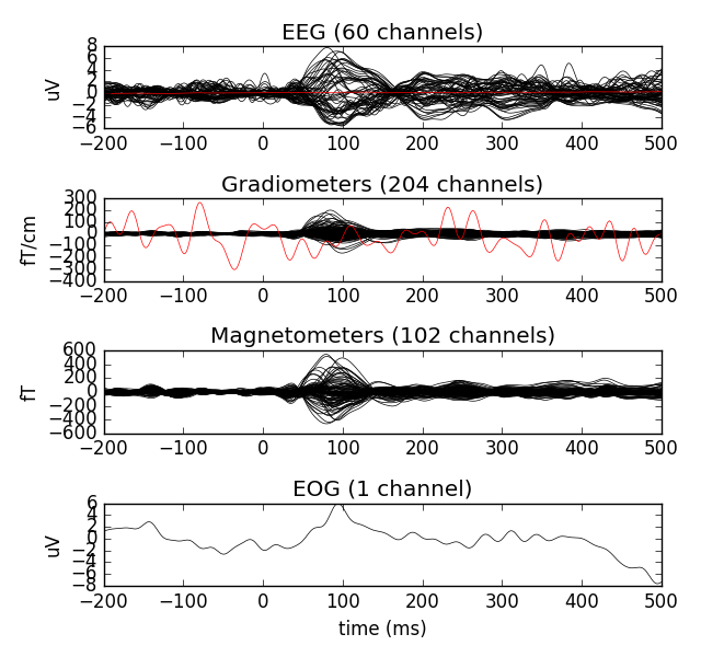
Let’s start with a simple one. We plot event related potentials / fields
(ERP/ERF). The bad channels are not plotted by default. Here we explicitly
set the exclude parameter to show the bad channels in red. All plotting
functions of MNE-python return a handle to the figure instance. When we have
the handle, we can customise the plots to our liking.
fig = evoked_l_aud.plot(exclude=())
All plotting functions of MNE-python return a handle to the figure instance. When we have the handle, we can customise the plots to our liking. For example, we can get rid of the empty space with a simple function call.
fig.tight_layout()
Now let’s make it a bit fancier and only use MEG channels. Many of the
MNE-functions include a picks parameter to include a selection of
channels. picks is simply a list of channel indices that you can easily
construct with mne.pick_types(). See also mne.pick_channels() and
mne.pick_channels_regexp().
Using spatial_colors=True, the individual channel lines are color coded
to show the sensor positions - specifically, the x, y, and z locations of
the sensors are transformed into R, G and B values.
picks = mne.pick_types(evoked_l_aud.info, meg=True, eeg=False, eog=False)
evoked_l_aud.plot(spatial_colors=True, gfp=True, picks=picks)
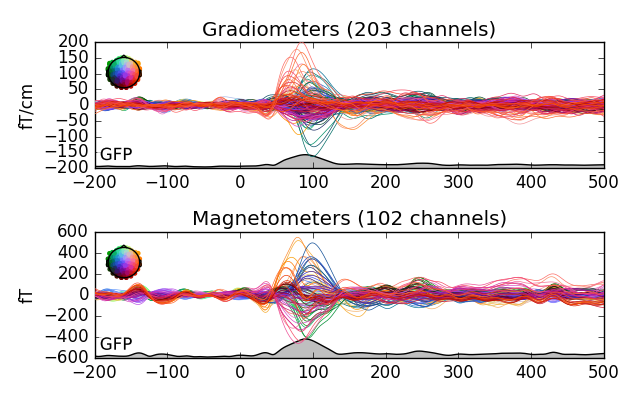
Notice the legend on the left. The colors would suggest that there may be two separate sources for the signals. This wasn’t obvious from the first figure. Try painting the slopes with left mouse button. It should open a new window with topomaps (scalp plots) of the average over the painted area. There is also a function for drawing topomaps separately.
evoked_l_aud.plot_topomap()
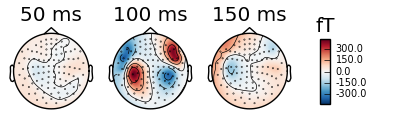
By default the topomaps are drawn from evenly spread out points of time over the evoked data. We can also define the times ourselves.
times = np.arange(0.05, 0.151, 0.05)
evoked_r_aud.plot_topomap(times=times, ch_type='mag')
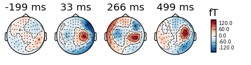
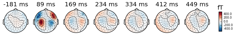
Or we can automatically select the peaks.
evoked_r_aud.plot_topomap(times='peaks', ch_type='mag')
You can take a look at the documentation of mne.Evoked.plot_topomap()
or simply write evoked_r_aud.plot_topomap? in your python console to
see the different parameters you can pass to this function. Most of the
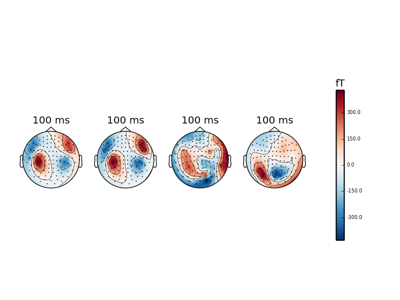
plotting functions also accept axes parameter. With that, you can
customise your plots even further. First we create a set of matplotlib
axes in a single figure and plot all of our evoked categories next to each
other.
fig, ax = plt.subplots(1, 5)
evoked_l_aud.plot_topomap(times=0.1, axes=ax[0], show=False)
evoked_r_aud.plot_topomap(times=0.1, axes=ax[1], show=False)
evoked_l_vis.plot_topomap(times=0.1, axes=ax[2], show=False)
evoked_r_vis.plot_topomap(times=0.1, axes=ax[3], show=True)
Out:
Colorbar is drawn to the rightmost column of the figure. Be sure to provide enough space for it or turn it off with colorbar=False.
Colorbar is drawn to the rightmost column of the figure. Be sure to provide enough space for it or turn it off with colorbar=False.
Colorbar is drawn to the rightmost column of the figure. Be sure to provide enough space for it or turn it off with colorbar=False.
Colorbar is drawn to the rightmost column of the figure. Be sure to provide enough space for it or turn it off with colorbar=False.
Notice that we created five axes, but had only four categories. The fifth
axes was used for drawing the colorbar. You must provide room for it when you
create this kind of custom plots or turn the colorbar off with
colorbar=False. That’s what the warnings are trying to tell you. Also, we
used show=False for the three first function calls. This prevents the
showing of the figure prematurely. The behavior depends on the mode you are
using for your python session. See http://matplotlib.org/users/shell.html for
more information.
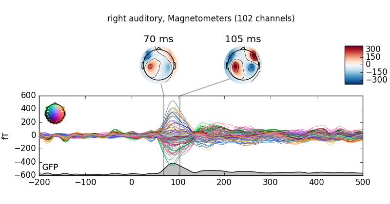
We can combine the two kinds of plots in one figure using the
mne.Evoked.plot_joint() method of Evoked objects. Called as-is
(evoked.plot_joint()), this function should give an informative display
of spatio-temporal dynamics.
You can directly style the time series part and the topomap part of the plot
using the topomap_args and ts_args parameters. You can pass key-value
pairs as a python dictionary. These are then passed as parameters to the
topomaps (mne.Evoked.plot_topomap()) and time series
(mne.Evoked.plot()) of the joint plot.
For an example of specific styling using these topomap_args and
ts_args arguments, here, topomaps at specific time points
(70 and 105 msec) are shown, sensors are not plotted (via an argument
forwarded to plot_topomap), and the Global Field Power is shown:
ts_args = dict(gfp=True)
topomap_args = dict(sensors=False)
evoked_r_aud.plot_joint(title='right auditory', times=[.07, .105],
                        ts_args=ts_args, topomap_args=topomap_args)


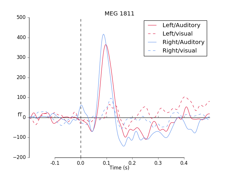
Sometimes, you may want to compare two or more conditions at a selection of
sensors, or e.g. for the Global Field Power. For this, you can use the
function mne.viz.plot_compare_evokeds(). The easiest way is to create
a Python dictionary, where the keys are condition names and the values are
mne.Evoked objects. If you provide lists of mne.Evoked
objects, such as those for multiple subjects, the grand average is plotted,
along with a confidence interval band - this can be used to contrast
conditions for a whole experiment.
First, we load in the evoked objects into a dictionary, setting the keys to
‘/’-separated tags (as we can do with event_ids for epochs). Then, we plot
with mne.viz.plot_compare_evokeds().
The plot is styled with dictionary arguments, again using “/”-separated tags.
We plot a MEG channel with a strong auditory response.
conditions = ["Left Auditory", "Right Auditory", "Left visual", "Right visual"]
evoked_dict = dict()
for condition in conditions:
    evoked_dict[condition.replace(" ", "/")] = mne.read_evokeds(
        fname, baseline=(None, 0), proj=True, condition=condition)
print(evoked_dict)

colors = dict(Left="Crimson", Right="CornFlowerBlue")
linestyles = dict(Auditory='-', visual='--')
pick = evoked_dict["Left/Auditory"].ch_names.index('MEG 1811')

mne.viz.plot_compare_evokeds(evoked_dict, picks=pick,
                             colors=colors, linestyles=linestyles)
Out:
Reading /home/ubuntu/mne_data/MNE-sample-data/MEG/sample/sample_audvis-ave.fif ...
    Read a total of 4 projection items:
        PCA-v1 (1 x 10²) active
        PCA-v2 (1 x 10²) active
        PCA-v3 (1 x 10²) active
        Average EEG reference (1 x 60) active
    Found the data of interest:
        t =    -199.80 ...     499.49 ms (Left Auditory)
        0 CTF compensation matrices available
        nave = 55 - aspect type = 100
Projections have already been applied. Setting proj attribute to True.
Applying baseline correction (mode: mean)
Reading /home/ubuntu/mne_data/MNE-sample-data/MEG/sample/sample_audvis-ave.fif ...
    Read a total of 4 projection items:
        PCA-v1 (1 x 10²) active
        PCA-v2 (1 x 10²) active
        PCA-v3 (1 x 10²) active
        Average EEG reference (1 x 60) active
    Found the data of interest:
        t =    -199.80 ...     499.49 ms (Right Auditory)
        0 CTF compensation matrices available
        nave = 61 - aspect type = 100
Projections have already been applied. Setting proj attribute to True.
Applying baseline correction (mode: mean)
Reading /home/ubuntu/mne_data/MNE-sample-data/MEG/sample/sample_audvis-ave.fif ...
    Read a total of 4 projection items:
        PCA-v1 (1 x 10²) active
        PCA-v2 (1 x 10²) active
        PCA-v3 (1 x 10²) active
        Average EEG reference (1 x 60) active
    Found the data of interest:
        t =    -199.80 ...     499.49 ms (Left visual)
        0 CTF compensation matrices available
        nave = 67 - aspect type = 100
Projections have already been applied. Setting proj attribute to True.
Applying baseline correction (mode: mean)
Reading /home/ubuntu/mne_data/MNE-sample-data/MEG/sample/sample_audvis-ave.fif ...
    Read a total of 4 projection items:
        PCA-v1 (1 x 10²) active
        PCA-v2 (1 x 10²) active
        PCA-v3 (1 x 10²) active
        Average EEG reference (1 x 60) active
    Found the data of interest:
        t =    -199.80 ...     499.49 ms (Right visual)
        0 CTF compensation matrices available
        nave = 58 - aspect type = 100
Projections have already been applied. Setting proj attribute to True.
Applying baseline correction (mode: mean)
{'Left/Auditory': <Evoked  |  comment : 'Left Auditory', kind : average, time : [-0.199795, 0.499488], n_epochs : 55, n_channels x n_times : 376 x 421, ~4.9 MB>, 'Left/visual': <Evoked  |  comment : 'Left visual', kind : average, time : [-0.199795, 0.499488], n_epochs : 67, n_channels x n_times : 376 x 421, ~4.9 MB>, 'Right/Auditory': <Evoked  |  comment : 'Right Auditory', kind : average, time : [-0.199795, 0.499488], n_epochs : 61, n_channels x n_times : 376 x 421, ~4.9 MB>, 'Right/visual': <Evoked  |  comment : 'Right visual', kind : average, time : [-0.199795, 0.499488], n_epochs : 58, n_channels x n_times : 376 x 421, ~4.9 MB>}
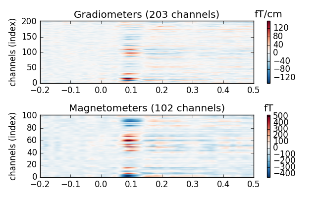
We can also plot the activations as images. The time runs along the x-axis
and the channels along the y-axis. The amplitudes are color coded so that
the amplitudes from negative to positive translates to shift from blue to
red. White means zero amplitude. You can use the cmap parameter to define
the color map yourself. The accepted values include all matplotlib colormaps.
evoked_r_aud.plot_image(picks=picks)
Finally we plot the sensor data as a topographical view. In the simple case we plot only left auditory responses, and then we plot them all in the same figure for comparison. Click on the individual plots to open them bigger.
title = 'MNE sample data (condition : %s)'
evoked_l_aud.plot_topo(title=title % evoked_l_aud.comment)
colors = 'yellow', 'green', 'red', 'blue'
mne.viz.plot_evoked_topo(evoked, color=colors,
                         title=title % 'Left/Right Auditory/Visual')


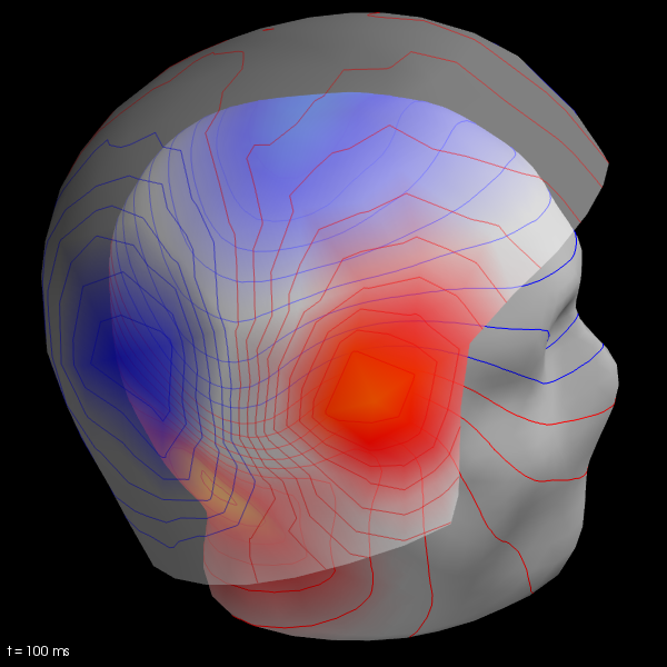
We now compute the field maps to project MEG and EEG data to MEG helmet and scalp surface.
To do this we’ll need coregistration information. See Head model and forward computation for more details.
Here we just illustrate usage.
subjects_dir = data_path + '/subjects'
trans_fname = data_path + '/MEG/sample/sample_audvis_raw-trans.fif'

maps = mne.make_field_map(evoked_l_aud, trans=trans_fname, subject='sample',
                          subjects_dir=subjects_dir, n_jobs=1)

# explore several points in time
field_map = evoked_l_aud.plot_field(maps, time=.1)
Out:
Using surface from /home/ubuntu/mne_data/MNE-sample-data/subjects/sample/bem/sample-5120-5120-5120-bem.fif.
Getting helmet for system 306m
Prepare EEG mapping...
Computing dot products for 59 electrodes...
Computing dot products for 2562 surface locations...
Field mapping data ready
    Preparing the mapping matrix...
    [Truncate at 20 missing 0.001]
    The map will have average electrode reference
Prepare MEG mapping...
Computing dot products for 305 coils...
Computing dot products for 304 surface locations...
Field mapping data ready
    Preparing the mapping matrix...
    [Truncate at 209 missing 0.0001]
Note
If trans_fname is set to None then only MEG estimates can be visualized.
Total running time of the script: ( 0 minutes 24.304 seconds)